Abstract

We present a fluid-dynamic model for the simulation of urban traffic networks with road sections of different lengths and capacities. The model allows one to efficiently simulate the transitions between free and congested traffic, taking into account congestion-responsive traffic assignment and adaptive traffic control. We observe dynamic traffic patterns which significantly depend on the respective network topology. Synchronization is only one interesting example and implies the emergence of green waves. In this connection, we will discuss adaptive strategies of traffic light control which can considerably improve throughputs and travel times, using self-organization principles based on local interactions between vehicles and traffic lights. Similar adaptive control principles can be applied to other queueing networks such as production systems. In fact, we suggest to turn push operation of traffic systems into pull operation: By removing vehicles as fast as possible from the network, queuing effects can be most efficiently avoided. The proposed control concept can utilize the cheap sensor technologies available in the future and leads to reasonable operation modes. It is flexible, adaptive, robust, and decentralized rather than based on precalculated signal plans and a vulnerable traffic control center.

[Self-Organized Control of Irregular or Perturbed Network Traffic]Self-Organized Control of
Irregular or Perturbed
Network Traffic

Self-Organized Control of Irregular or Perturbed Network Traffic

1 Introduction

Traffic control in networks has a long history. Early efforts have aimed at synchronizing traffic signals along a one-way, then a two-way arterial. There is still potential for improvement in this direction, as is attested by some recent research efforts [Stamatiadis and Gartner (1999)] or prompted by the development of new theoretical tools [Lotito et al. (2002), Mancinelli et al. (2001)]. Synchronization of traffic along arterials results in so-called green-waves, the aim of which is simply to ensure that traffic flows smoothly along main streets. Expected benefits of green waves are reduced fuel consumption and travel times.

The green-wave approach can be generalized to networks, yielding pre-calculated signal control schemes, such as TRANSYT [Robertson (1997)]. In principle such schemes are completely coercive: they force the traffic flow to comply with pre-calculated patterns, optimizing such criteria as the total travel time spent. Since traffic demand varies, the need for some responsiveness of the signal control was felt very soon. The SCOOT system [Robertson and Bretherton (1991)], an outgrowth of TRANSYT, allows for smooth change in the signal settings in response to changes in the traffic demand.

Among the strategies making use of precalculated controls, let us mention SCATS [Sims and Dobinson (1979), Lin and Chen (2004)], which relies on a library of controls (green durations, offsets, …) according to traffic conditions. Even the optimization criterion depends on the traffic state. The system might, at night, minimize the number of stops, maximize throughput at day time under normal conditions, and aim at postponing the onset of congestion under heavy traffic conditions.

More recent developments stress greater adaptability. For instance UTOPIA [Mauro and Di Taranto (1989)] combines a regional control based on prediction of traffic flow through the main network arteries with the action of local intersection controllers. The regional control simply serves as a reference for local control.

OPAC [Gartner (1990)] optimizes queues in accordance with the “store-and-forward” concept [Papageorgiou (1991)], based on dynamic programming, with a rolling horizon. OPAC is fundamentally designed to manage intersections but extends to networks.

Even more decentralized and demand-responsive at a very local level, PRODYN [Henry and Farges (1989)] optimizes traffic at intersections by switching traffic lights on a traffic-actuated basis. Optimality is achieved through the dynamic programming technique. PRODYN also tries to coordinate neighboring intersections.

A further development includes dynamic assignment into the calculation of optimal traffic light settings as well as non-mandatory management schemes (user information). METACOR [Elloumi et al. (1994)], based on an optimal control strategy with a rolling horizon, is a good example of this approach. In the same line of approach, TUC [Diakaki et al. (2003)] displays two innovative features:

• a reference strategy is calculated for the network (for a given situation),

• a filter is included into the algorithm which calculates the commands. The aim of the filter is to detect and adjust deviations from the nominal traffic situation, and also to detect in real time deviations in parameter values.

A notable trend in recent research on demand-responsive traffic management systems is greater reliance on artificial intelligence (AI) methods, prompted by an ever growing complexity of algorithms, models and data. Let us cite some examples of this trend: [Li et al. (2004), Sayers et al. (1998), Niittymäki (2002)] and CLAIRE [Scémama (1994)].

Overall, no matter how sophisticated these classical approaches,

• either their responsiveness is limited and they appear as tools both coercive and normative (imposing a traffic situation rather than responding to it),

• or they are completely demand-responsive (CLAIRE or PRODYN for instance) and lack a global coordination. The TUC strategy might be viewed as a nice compromise.

All classical approaches require vast amounts of data collection and processing, as well as huge processing power. Further, global coordination notoriously requires data difficult to obtain or elaborate such as dynamic origin-destination matrices or dynamic assignment data. Finally, the systems described so far have a difficult time responding to exceptional events, accidents, temporary building sites or other changes in the road network, natural or industrial disasters, catastrophes, terrorist attacks etc.

Hence the usefulness of the decentralized and self-organized approach advocated in this paper is its greater degree of flexibility, its independence of a central traffic control center, and its greater robustness with respect to local perturbations or failures. As shown in Sec. 4 and summarized in Sec. 5, our autonomous adaptive control based on a traffic-responsive self-organization of traffic lights leads to reasonable operations, including synchronization patterns such as green waves. In particular, our principle of self-control is suited for irregular (i.e. non-Manhattan type) road networks with counterflows, with main roads (arterials) and side roads, with varying inflows, and with changing turning or assignment fractions. This distinguishes our approach from simplified scenarios investigated elsewhere [Brockfeld et al. (2001), Fouladvand and Nematollahi (2001), Huang and Huang (2003)]. Another interesting feature is that our approach considers not only “pressures” on the traffic lights related to delay times. It also takes into account “counter-pressures” when subsequent road sections are full, i.e. when green times cannot be effectively used.

2 Modeling traffic flow in urban road networks

In our model of urban road traffic, road networks are composed of nodes (intersections, plazas, dead ends, or cross sections of the road), which are connected by directed links $i$, representing homogeneous road sections without changes in capacity.

2.1 Traffic flow on network links

Figure 1: A road network (a) can be considered as a directed graph (b). The directed links represent homogeneous road sections, while the nodes correspond to junctions. (c) The road sections may or may not be controlled by traffic lights.

2.1.1 Homogeneous road sections

Our road sections $i$ are characterized by a constant number $I_{i}$ of lanes, over which traffic is assumed to be equally distributed. Different lanes turning into different directions may be treated as separate road sections, depending on the respective design of the infrastructure. Road sections can have a very large length $L_{i}$, which is in favor of numerical efficiency. The dynamics within a link of the road network is described by the section-based queueing-theoretical traffic model by Helbing (2003b). It is directly related to the equation of vehicle conservation [Lighthill and Whitham (1955)] and briefly introduced, here. The average velocity of vehicles on link $i$ around place $x$ at time $t$ is denoted by $V_{i}(x,t)$, the spatial density per lane by $\rho_{i}(x,t)$, and the flow per lane by $Q_{i}(x,t)=\rho_{i}(x,t)V_{i}(x,t)$. The flow is approximated by a triangular flow-density relationship

$$Q_{i}(x,t)=\left\{\begin{array}[]{ll}\rho_{i}(x,t)V_{i}^{0}&\mbox{if }1/\rho_{i}(x,t)>\left(1/\rho^{\rm jam}+TV_{i}^{0}\right)\\ \frac{1}{T}\left[1-\rho_{i}(x,t)/\rho^{\rm jam}\right]&\mbox{otherwise (in congested traffic).}\end{array}\right.$$ (1)

While the increasing line $\rho_{i}V_{i}^{0}$ describes free traffic moving with speed $V_{i}^{0}$, the falling “jam line” describes congested traffic, in which the average vehicle distance $1/\rho_{i}$ is given by an effective vehicle length $l^{\rm eff}=1/\rho^{\rm jam}$ (= vehicle length plus minimum front-bumper-to-back-bumper distance) plus a safety distance $TV_{i}$ which grows linearly with the speed $V_{i}$. The proportionality factor is the (safe) time gap $T$ kept in congested traffic. Therefore, our model is based on only three intuitive parameters: the maximum jam density $\rho^{\rm jam}$, the free velocity $V_{i}^{0}$ (speed limit) on link $i$, and the time gap in congested traffic $T$. In our paper, we have chosen $V_{i}^{0}=14\mbox{ m/s}=50$ km/h, $\rho^{\rm jam}=150$ vehicles per kilometer and lane, and $T=1.8$ s.

We should note that there are other macroscopic traffic models such as the non-local, gas-kinetic-based traffic (GKT) model [Treiber at al. (1999)], which can describe the aggregate dynamics of traffic flows more accurately than this model. The “GKT model” has even been successfully implemented to simulate traffic flows on all German freeways, taking into account information by local detectors and floating car data. However, the dynamics of urban traffic is dominated by the dynamics of the traffic lights, which justifies simplifications in favor of numerical efficiency and analytical treatment. The section-based traffic model covers the most essential features of traffic flow in urban road networks, e.g. the transition between free and congested traffic, the spreading and interaction of vehicle queues, etc. Its particular strengths are its transparency, numerical stability, and computational efficiency. Compared to microsimulation models of urban traffic such as cellular automata models [Cremer and Ludwig (1986), Esser and Schreckenberg (1997), Nagel et al. (2000)], the treatment of lane changes, intersections, and turning operations is much easier, and analytical investigations are possible.

2.1.2 Propagation of perturbations

The particular simplicity of the section-based traffic model results from its two constant characteristic velocities: While perturbations of free traffic propagate together with the cars at the speed $V_{i}^{0}$, in congested traffic perturbations travel upstream with the constant velocity

$$c=-1/(T\rho^{\rm jam})\,,$$ (2)

which has the typical value of $-3.7$ m/s or $-13.3$ km/h.

A favorable property of the section-based traffic model is that all relevant quantities can be determined from the boundary flows, which makes the model very efficient. For example, the dynamics inside a road section $i$ can be easily derived from the arrival flow $Q_{i}^{\rm arr}(t)$ and the departure flow $Q_{i}^{\rm dep}(t)$ per lane with the two characteristic velocities $V_{i}^{0}$ and $c$, see Fig. 2.

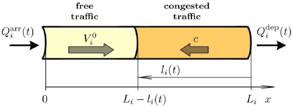
Figure 2: A road section $i$ of length $L_{i}$ with an area $l_{i}$ of congested traffic at the downstream end (right). Due to the constant propagation speeds $V_{i}^{0}$ and $c$ of perturbations in free and congested traffic, respectively (see big arrows), the internal dynamics can be easily calculated based on the boundary flows $Q_{i}^{\rm arr}(t)$ and $Q_{i}^{\rm dep}(t)$ only.

The interior flow per lane is given by

$$Q_{i}(x,t)=\left\{\begin{array}[]{ll}Q_{i}^{\rm arr}\left(t-\frac{x}{V_{i}^{0}}\right)&\mbox{if }x<L_{i}-l_{i}(t)\mbox{ (in free traffic)}\,,\\ Q_{i}^{\rm dep}\left(t-\frac{L_{i}-x}{|c|}\right)&\mbox{if }L_{i}-l_{i}(t)\leq x\leq L_{i}.\end{array}\right.$$ (3)

That is, the flow is determined by the downstream boundary in the area of congested traffic of length $l_{i}(t)\geq 0$, while it is given by the arrival flow in the area $x<L_{i}-l_{i}(t)$ of free traffic. The density can be obtained via

$$\rho_{i}(x,t)=\left\{\begin{array}[]{ll}Q_{i}(x,t)/V_{i}^{0}&\mbox{if }x<L_{i}-l_{i}(t)\mbox{ (in free traffic)}\,,\\ {[1-TQ_{i}(x,t)]}\rho^{\rm jam}&\mbox{if }L_{i}-l_{i}(t)\leq x\leq L_{i}.\end{array}\right.$$ (4)

The average velocity is calculated via the formula $V_{i}(x,t)=Q_{i}(x,t)/\rho_{i}(x,t)$, if $\rho_{i}(x,t)>0$.

The temporal change of the number $N_{i}(t)$ of vehicles per lane on road section $i$ can be also determined from the arrival and departure flows:

$$\frac{dN_{i}}{dt}=Q_{i}^{\rm arr}(t)-Q_{i}^{\rm dep}(t)\,.$$ (5)

The time-dependent change of the congested area of length $l_{i}(t)$ will be discussed in the next paragraph.

2.1.3 Movement of congestion fronts

Since our road sections are homogeneous by definition, congestion can only be triggered at their downstream ends. While the congested area might eventually expand over the entire road section, the downstream end remains at $x=L_{i}$. The upstream end lies at $x=L_{i}-l_{i}(t)$, where jumps $\Delta\rho_{i}$ and $\Delta Q_{i}$ occur in the density and in the flow, respectively. In order to ensure the conservation of vehicles, the condition $\Delta Q_{i}=-\Delta\rho_{i}\cdot dl_{i}/dt$ must be fulfilled. Therefore, the border line between free and congested traffic moves with the following velocity [Helbing (2003b)]:

$$\frac{dl_{i}}{dt}\;=\;-\;\frac{Q_{i}^{\rm arr}\big{(}t-[L_{i}-l_{i}(t)]/V_{i}^{0}\big{)}-Q_{i}^{\rm dep}\big{(}t-l_{i}(t)/|c|\big{)}}{\rho_{i}^{\rm arr}\;\big{(}t-[L_{i}-l_{i}(t)]/V_{i}^{0}\big{)}-\rho_{i}^{\rm dep}\;\big{(}t-l_{i}(t)/|c|\big{)}}\;.$$ (6)

Note that, within the congested area of length $l_{i}(t)$, one might find areas of quasi-free traffic, where the vehicles reach the maximum free velocity $V_{i}^{0}$ and the maximum flow $Q_{i}^{\rm max}$ per lane that is possible according to the flow-density relationship (1):

$$Q_{i}^{\rm max}=\left(T+\frac{1}{V_{i}^{0}\rho^{\rm jam}}\right)^{-1}\,.$$ (7)

This value corresponds to vehicles accelerating out of a traffic jam every $T=1.8$ seconds. Nevertheless, the value $1/T$ is not completely reached, as each subsequent vehicle has to drive an additional distance $l^{\rm eff}=1/\rho^{\rm jam}$ in order to reach the respective measurement cross section. This requires an additional time interval of $l^{\rm eff}/V_{i}^{0}$ as in the formula above (see Fig. 3).

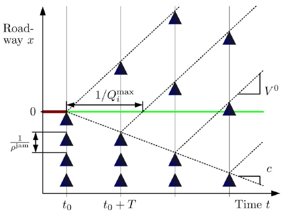
Figure 3: Illustration of queued vehicles (triangles in the lower left corner) and freely moving vehicles after a traffic light turns green (triangles in the upper right part). The characteristic speeds $V^{0}$ and $c$ are indicated by diagonal lines.

Let us shortly discuss two special cases of formula (6): If the departure flow is stopped due to a red traffic light, we obtain the simplified relationship

$$\frac{dl_{i}}{dt}=\left[\frac{\rho^{\rm jam}}{Q_{i}^{\rm arr}\left(t-[L_{i}-l_{i}(t)]/V_{i}^{0}\right)}-\frac{1}{V_{i}^{0}}\right]^{-1}\approx\frac{Q_{i}^{\rm arr}\left(t-[L_{i}-l_{i}(t)]/V_{i}^{0}\right)}{\rho^{\rm jam}}\,.$$ (8)

If the traffic light turns green at time $t^{\prime}_{0}$, the end of the traffic jam still propagates upstream at the speed (8) with new arriving vehicles. However, at the same time, an area of quasi-free traffic with maximum flow $Q_{i}^{\rm max}$ propagates upstream with velocity $c$ from the downstream boundary. Therefore, the effective length $l_{i}^{\rm eff}(t)$ of the vehicle queue is

$$l_{i}^{\rm eff}(t)=l_{i}(t)-|c|(t-t^{\prime}_{0})\,.$$ (9)

If this effective queue has been fully resolved at time $t^{*}$, i.e. $l_{i}^{\rm eff}(t^{*})=0$, it takes an additional time $l_{i}(t^{*})/V_{i}^{0}$ until the last vehicle of that queue has left the road section $i$. Therefore, we reach $l_{i}(t)=0$ and, thereby, free traffic on the whole road section $i$, at time $t^{*}+l_{i}(t^{*})/V_{i}^{0}$. Before this point in time, vehicles that have moved out of the queue may still be trapped again by a red traffic light at the end of road section $i$.

2.1.4 Travel time

Let the travel time $T_{i}(t)$ be the time a vehicle needs to pass through the road section $i$ when entering it at time $t$. Then, the actual number $N_{i}(t)$ of vehicles inside the road section is given by

$$N_{i}(t)=\!\!\int\limits_{t}^{t+T_{i}(t)}\!\!dt^{\prime}\;Q_{i}^{\rm dep}(t^{\prime})\,.$$ (10)

This formula implies the following delay-differential equation describing how the travel time $T_{i}$ depends on the boundary flows [Helbing (2003b)]:

$$\frac{dT_{i}}{dt}=\frac{Q_{i}^{\rm arr}(t)}{Q_{i}^{\rm dep}\big{(}t+T_{i}(t)\big{)}}-1\,.$$ (11)

According to this, the travel time can be predicted based on the anticipated departure flow, e.g. when a certain traffic light control is assumed (see Secs. 2.1.5 and 4.3).

2.1.5 Delay time

Since the travel time would exactly be $L_{i}/V_{i}^{0}$ without congestion, any deviation from that can be understood as the time a vehicle has been delayed due to congestion. Therefore, we may introduce the delay time

$$T_{i}^{\rm del}(t)=T_{i}-\frac{L_{i}}{V_{i}^{0}}\,.$$ (12)

Since $L_{i}/V_{i}^{0}$ is time-independent, the right hand side of equation (11) applies to $dT_{i}^{\rm del}/dt$ as well.

Consider a road section with a constant arrival flow $Q_{i}^{\rm arr}(t)$ and a departure flow $Q_{i}^{\rm dep}(t)=\gamma_{i}(t)Q_{i}^{\rm max}$ being controlled by a traffic light. As the buffer size is given by the maximum number $L_{i}\rho^{\rm jam}$ of vehicles per lane on road section $i$, from Eq. (5) we can derive

$$\frac{1}{t}\int\limits_{0}^{t}dt^{\prime}\;Q_{i}^{\rm arr}(t^{\prime}) \leq \frac{L_{i}\rho^{\rm jam}}{t}+\frac{1}{t}\int\limits_{0}^{t}dt^{\prime}\;Q_{i}^{\rm dep}(t^{\prime})$$ (13)

$$\leq \frac{L_{i}\rho^{\rm jam}}{t}+\frac{Q_{i}^{\rm max}}{t}\int\limits_{0}^{t}dt^{\prime}\;\gamma_{i}(t^{\prime})$$

$$= \frac{L_{i}\rho^{\rm jam}}{t}+u_{i}Q_{i}^{\rm max}$$

with the average green time fraction

$$u_{i}=\frac{1}{t}\int\limits_{0}^{t}dt^{\prime}\;\gamma_{i}(t^{\prime})\,.$$ (14)

For $t\rightarrow\infty$ we can see that the average arrival rate per lane on road section $i$ should not exceed the maximum flow times the green time fraction $u_{i}$. Otherwise, we will have a growing queue, until the maximum storage capacity $I_{i}L_{i}\rho^{\rm jam}$ for vehicles on road section $i$ has been reached.

The throughput is reduced if a downstream road section $j$ is sometimes fully congested, as this limits the departure flow. Moreover, the delay time can temporarily increase, if the arrival of vehicles at the upstream boundary of road section $i$ is not synchronized with the green phase of the traffic light at the downstream end. Such a synchronization of arrivals in $i$ with the desired departure times is hard to reach in an irregular road network. As a consequence, vehicles tend to queue up at a red light before they can leave a road section $i$ (see Fig. 4). Note, however, that a green light reaches maximum efficiency when it serves vehicles which have queued up before.

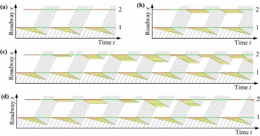
Figure 4: Trajectories of freely moving vehicles (diagonal lines) and queued vehicles (horizontal lines) in dependence of the traffic light control at two subsequent intersections 1 and 2. In all four displayed scenarios, vehicles arrive with identical time headways (i.e. constant arrival rate) at traffic light 1, which operates periodically. Traffic light 2 is operated in different modes: (a) The frequency and time offset are adapted to the first traffic light, as required by a green wave. (b) The frequency is the same as for the first traffic light, but has a non-optimal time offset. (c) The frequency (and cycle time) differs from the one of the first traffic light. (d) The green time varies stochastically, but the average green time fraction is the same. When the frequencies are the same, but the time offset is not properly adjusted, a certain fraction of vehicles is stopped, see (b). If the frequencies are different, it is most likely that vehicles will be stopped by a red light, potentially even for several times, see (c). In such cases, a stochastic variation of green time periods can be favorable, see (d).

Let us now study the case where the waiting queues cannot be cleared completely within one green phase. How long is a vehicle delayed, if it joins a queue of length $l_{i}(t_{0})$ at time $t_{0}$? The totally required green time needed until the vehicle can leave the road section $i$ is given by

$$T_{i}^{\rm req}(t_{0})=\frac{l_{i}(t_{0})\rho^{\rm jam}}{Q_{i}^{\rm max}}\,,$$ (15)

since $l_{i}(t_{0})\rho^{\rm jam}$ is the number of vehicles per lane to be served and $Q_{i}^{\rm max}$ the service rate. Let us now estimate the overall time passed until the downstream boundary of road section $i$ is reached. It is given by the formula

$$T_{i}^{\rm pass}(t_{0})=T_{i}^{\rm req}(t_{0})+\mbox{overall red and yellow times in between.}$$ (16)

The time delay of vehicle $i$ by queuing, red and yellow times is the overall time passed minus the travel time $l_{i}(t_{0})/V_{i}^{0}$ in free traffic:

$$T_{i}^{\rm del}(t_{0}) = T_{i}^{\rm pass}-\frac{l_{i}(t_{0})}{V_{i}^{0}}$$

$$= l_{i}(t_{0})\left(\frac{\rho^{\rm jam}}{Q_{i}^{\rm max}}-\frac{1}{V_{i}^{0}}\right)+\mbox{overall red and yellow times.}$$

Generally, this formula is difficult to express, as its result depends sensitively on the respective red and green phases. However, the formula for the average delay time becomes quite simple. Just remember that the average green time fraction is $u_{i}$ and the average fraction of red and yellow times must be $1-u_{i}$. Therefore, the average delay $\overline{T_{i}^{\rm del}}$ as a function of the average queue length $\overline{l_{i}}$ and the green time fraction $u_{i}$ is estimated by the formula

$$\overline{T_{i}^{\rm del}} \approx \overline{l_{i}}\left(\frac{\rho^{\rm jam}}{Q_{i}^{\rm max}}-\frac{1}{V_{i}^{0}}\right)+\frac{1-u_{i}}{u_{i}}\times\mbox{totally required green time }T_{i}^{\rm req}$$ (18)

$$= \overline{l_{i}}\left(\frac{\rho^{\rm jam}}{u_{i}Q_{i}^{\rm max}}-\frac{1}{V_{i}^{0}}\right)\,.$$

According to this, the average delay time $\overline{T_{i}^{\rm del}}$ is proportional to the average queue length $\overline{l_{i}}$, but a large green time fraction $u_{i}$ is helpful. Note that the formulas of this section are not only applicable to situations with fixed cycle times and signal programs. They are also applicable to situations where the red and green phases are varying.

2.1.6 Potential flows and traffic states

The in- and outflow of a road section is not only limited by capacity constraints such as $Q_{i}^{\rm max}$, but also by the actual state of traffic. We will, therefore, denote the potential arrival and departure flows per lane by $Q_{i}^{\rm arr,pot}(t)$ and $Q_{i}^{\rm dep,pot}(t)$, respectively. Congestion is triggered if $Q_{i}^{\rm dep}(t)>Q_{i}^{\rm dep,pot}(t)$, and resolved if $l_{i}(t)=0$. In the case where the road section is entirely congested, i.e. $l_{i}(t)=L_{i}$, this state remains until $Q_{i}^{\rm arr}(t)<Q_{i}^{\rm arr,pot}(t)$. The potential flows are determined as follows: As long as there is no congestion, the potential departure flow is given by the former arrival flow $Q_{i}^{\rm arr}(t-L_{i}/V_{i}^{0})$. When the downstream end of road section $i$ is congested, vehicles are queued up and can depart with the maximum possible flow $Q_{i}^{\rm max}$. Altogether, we have

$$Q_{i}^{\rm dep,pot}(t)=\left\{\begin{array}[]{ll}Q_{i}^{\rm arr}(t-L_{i}/V_{i}^{0})&\mbox{if }l_{i}(t)=0\,,\\ Q_{i}^{\rm max}&\mbox{if }l_{i}(t)>0\,.\end{array}\right.$$ (19)

At the upstream end, the maximum possible flow $Q_{i}^{\rm max}$ can enter road section $i$ as long as it is not entirely congested. Otherwise, the arrival flow is limited by the former departure flow $Q_{i}^{\rm dep}(t-L_{i}/|c|)$. This implies

$$Q_{i}^{\rm arr,pot}(t)=\left\{\begin{array}[]{ll}Q_{i}^{\rm max}&\mbox{if }l_{i}(t)<L_{i}\,,\\ Q_{i}^{\rm dep}(t-L_{i}/|c|)&\mbox{if }l_{i}(t)=L_{i}\,.\end{array}\right.$$ (20)

In cases, where the outflow of the road section is to be controlled by a traffic light, the potential departure flow $Q_{i}^{\rm dep,pot}(t)$ must be multiplied with a prefactor $\gamma_{i}(t)$. A green light corresponds to $\gamma_{i}(t)=1$, a red light to $\gamma_{i}(t)=0$. Note that it is also possible to vary $\gamma_{i}(t)$ gradually to account for drivers passing the signal during yellow phases.

2.2 Traffic flows through network nodes

A node of the road network connects one or several incoming road sections $i$ with one or several outgoing road sections $j$, see figure 5(a). It may represent a junction or a link of two subsequent homogeneous road sections $i$ and $i+1$ with different speed limits $V_{i}^{0}$, $V_{i+1}^{0}$ or numbers $I_{i}$, $I_{i+1}$ of lanes. Since nodes are assumed to have no storage capacity, the total in- and outflow have to be the same (Kirchhoff’s law):

$$\underbrace{\Big{.}\sum\nolimits_{i}Q_{i}^{\rm dep}(t)}_{\rm inflow}=\underbrace{\Big{.}\sum\nolimits_{j}Q_{j}^{\rm arr}(t)}_{\rm outflow}\,.$$ (21)

Furthermore, the flows have to be non-negative and must not exceed the potential flows specified in Sec. 2.1.6.

$$0\leq Q_{i}^{\rm dep}(t)\leq Q_{i}^{\rm dep,pot}(t)\,,\qquad 0\leq Q_{j}^{\rm arr}(t)\leq Q_{j}^{\rm arr,pot}(t)\,.$$ (22)

The fraction of the inflow $Q_{i}^{\rm dep}$ that diverges from road section $i$ to road section $j$ is denoted by $\alpha_{ij}(t)$. Due to normalization we have

$$\sum_{j}\alpha_{ij}(t)=1\,.$$ (23)

The turning or assignment coefficients $\alpha_{ij}$ may depend on the driver destinations $d$ as well as on the actual traffic situation, see Daganzo (1995) and Sec. 3. Finally, note that the arrival flow $Q_{j}^{\rm arr}(t)$ is composed of all turning flows $Q_{i}^{\rm dep}(t)\alpha_{ij}(t)$ entering road section $j$:

$$Q_{j}^{\rm arr}(t)=\sum_{i}Q_{i}^{\rm dep}(t)\alpha_{ij}(t)\,.$$ (24)

For a more detailed treatment of network nodes see Lebacque (2005).

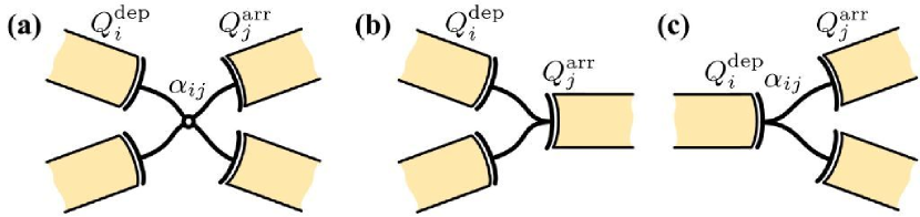
Figure 5: (a) A node of the road network distributes the vehicular flows between the road sections that are connected to it. It makes sense to distinguish two special cases: (b) merges into a single road section and (c) diverges from one road section into several others.

2.2.1 Merges

In the case where traffic flows from several incoming road sections $i$ merge into one outgoing road section $j$, as shown in Fig. 5(b), two cases can be distinguished: As long as the subsequent road section $j$ has sufficient capacity to admit the potential flows of all incoming road sections $i$, i.e. $Q_{j}^{\rm arr,pot}(t)\geq\sum_{i}Q_{i}^{\rm dep,pot}(t)$, the flow through the node is given by the upstream traffic conditions in the road sections $i$. Otherwise, some of the upstream departure flows $Q_{i}^{\rm dep}(t)$ have to be restricted. But which ones? According to practical experience, small traffic flows $Q_{i}^{\rm dep}(t)$ can almost always squeeze in, while flows from equivalent roads tend to share the capacity $Q_{j}^{\rm arr,pot}$ equally. Note that in scenarios with main roads having a right of way, the corresponding flow is to be served first. The remaining capacity is subsequently distributed among the side roads.

2.2.2 Diverges

Figure 5(c) shows the case where traffic diverges from one road section into several others. This is, for example, the case when a road splits up into lanes for turning left, continuing straight ahead, or turning right. For diverges, the throughput is determined by a cascaded minimum-function:

$$Q_{i}^{\rm dep}(t)=\min\left\{Q_{i}^{\rm dep,pot}(t),\;\;\min_{j}\frac{Q_{j}^{\rm arr,pot}(t)}{\alpha_{i{j}}(t)}\right\}\,.$$ (25)

The first term on the right-hand side is obvious, as any restriction of the potential departure flow $Q_{i}^{\rm dep,pot}(t)$ of road section $i$ limits the flows to all outgoing road sections $j$. The second term on the right-hand side follows from the fact that the fraction $\alpha_{ij}$ of the departure flow $Q_{i}^{\rm dep}(t)$ to any subsequent road section $j$ is limited by its potential arrival flow $Q_{j}^{\rm arr,pot}(t)$, i.e.

$$Q_{i}^{\rm dep}(t)\alpha_{ij}\leq Q_{j}^{\rm arr,pot}(t)\quad\forall j\,.$$ (26)

In the special case of a node connecting only two subsequent road sections $i$ and $j=i+1$, we have $\alpha_{ij}=1$ and the throughput is just limited by the minimum of both potential flows:

$$Q_{i}^{\rm dep}(t)=\min\Big{\{}Q_{i}^{\rm dep,pot}(t),\;\;Q_{i+1}^{\rm arr,pot}(t)\Big{\}}=Q_{i+1}^{\rm arr}(t)\,.$$ (27)

The last equality follows from Eq. (24).

3 Traffic assignment

The simplest way to model turning at intersections is by turning coefficients $\alpha_{ij}(t)$, which assume that a certain fraction $\alpha_{ij}(t)$ of the departure flow $Q_{i}^{\rm dep}(t)$ turns into road section $j$. In many theoretical studies, the coefficients $\alpha_{ij}$ are kept constant. However, it is well-known that the turning fractions vary in the course of the day, which is often taken into account by using historical, time-dependent turning coefficients $\alpha_{ij}(t)$ from a database [Chrobok et al. (2000)]. Moreover, even if the same origin-destination flows would repeat each week, delays due to perturbations in the traffic flow (e.g. due to an accident) would cause different time-dependent turning fractions. Therefore, a better treatment is based on dynamic traffic assignment.

In order to integrate dynamic traffic assignment in our model, let us denote the destination node of vehicles by $d$. Moreover, let $N_{id}(t)$ represent the number of driver-vehicle units on the directed link $i$, which finally want to arrive at $d$. This implies

$$N_{i}(t)=\sum_{d}N_{id}(t)\,.$$ (28)

The quantity $Q_{id}^{\rm arr}(t)$ shall denote the flow of vehicles with destination $d$ entering the link $i$, and $Q_{id}^{\rm dep}(t)$ the flow of vehicles leaving it. We have

$$Q_{i}^{\rm arr}(t)=\sum_{d}Q_{id}^{\rm arr}(t)\quad\mbox{and}\quad Q_{i}^{\rm dep}(t)=\sum_{d}Q_{id}^{\rm dep}(t)\,.$$ (29)

Finally, let $\overline{j}$ be the starting node of link $j$ and $\underline{j}=k$ its ending node. Moreover, let $T_{\overline{j}k}(t)$ be the travel time on link $j$ and $\widehat{T}_{kd}(t)$ the minimum travel time between two nodes $k$ and $d$ (as can, for example, be determined by the Dijkstra algorithm). Then, the minimum travel time to note $d$ via link $j$ (i.e. node $k$) is given by $T_{\overline{j}k}(t)+\widehat{T}_{kd}(t)$, and the minimum travel time $\widehat{T}_{\overline{j}d}(t)$ from node $\overline{j}$ to destination $d$ at time $t$ is determined via

$$\widehat{T}_{\overline{j}d}(t)=\min_{k}[T_{\overline{j}k}(t)+\widehat{T}_{kd}(t)]\,,$$ (30)

where the minimum function extends over all successors $k$ of node $\overline{j}$. Instead of this, we may use the following approximate relationship:

$$\widehat{T}_{\overline{j}d}(t)=\min_{k}[T_{\overline{j}k}(t)+\widehat{T}_{kd}(t-\Delta t)]\,.$$ (31)

The advantage of (31) over (30) is that the information about travel times gradually propagates to the present location of the car (namely by one link each time step $\Delta t$). A delayed evaluation of Dijkstra’s shortest path algorithm saves computer time and models this information flow, the speed of which is controlled by $\Delta t$. Another advantage is the determination of travel times based on a local algorithm.

Based on this travel time information, we may distribute the departure flows $Q_{i}^{d,{\rm dep}}(t)$ over neighboring links according to a multinomial logit model [Ben-Akiva, McFadden et al. (1999)]. Accordingly, we specify the turning probabilities of cars with destination $d$ at node $\overline{j}=\underline{i}$ as

$$p_{\overline{j}k}^{d}(t)=\frac{\mbox{exp}\{-\beta[T_{\overline{j}k}(t)+\widehat{T}_{kd}(t-\Delta t)]/\widehat{T}_{\overline{j}d}^{0}\}}{\sum_{k^{\prime}}\mbox{exp}\{-\beta[T_{\overline{j}k^{\prime}}(t)+\widehat{T}_{k^{\prime}d}(t-\Delta t)]/\widehat{T}_{\overline{j}d}^{0}\}}\,,$$ (32)

where $\widehat{T}_{\overline{j}d}^{0}$ is the minimum travel time from $\overline{j}$ to $d$ during free traffic (at three o’clock during the night). The coefficient $\beta$ describes the sensitivity with respect to changes in the relative travel time and is also a measure for the reliability of travel time estimates. Finally, the time-dependent assignment coefficients can be calculated as

$$\alpha_{ij}(t)=\sum_{d}\frac{Q_{id}^{\rm dep}(t)}{Q_{i}^{\rm dep}(t)}\,p_{\underline{i}\underline{j}}^{d}(t)\,,$$ (33)

where $\underline{i}=\overline{j}$ and $\underline{j}=k$. This assumes individual route choice decisions without central coordination, i.e. selfish routing.

We must still decide how to determine travel times. On the one hand, one may use the expected travel times $T_{\overline{j}k}(t)=T_{\overline{j}\underline{j}}(t)=T_{j}(t)$ according to Eq. (11) (or, as a second best alternative, the instantanous link travel times). On the other hand, one may use travel time information $T_{\overline{j}k}^{*}(t)$ of comparable days from a database [Chrobok et al. (2000)]. While for close links, the expected travel time may be a good (and the instantaneous travel time a reasonable) estimate of the actual travel time, it becomes less reliable the more remote the respective link is. For remote links, a travel time estimate based on measurements of similar previous days may be more reliable. Therefore, we propose to use a weighted mean value generalizing formula (31):

$$\widehat{T}_{\overline{j}d}(t)=\min_{k}[T_{\overline{j}k}(t)+\mbox{e}^{-\lambda\,T_{\overline{j}k}(t)}\widehat{T}_{kd}(t-\Delta t)+(1-\mbox{e}^{-\lambda\,T_{\overline{j}k}(t)})T_{kd}^{*}(t)]\,.$$ (34)

In this formula, the travel time $T_{kd}^{*}(t)$ from node $k$ to $d$ is taken from a database, the weights are exponentially decaying with increasing travel times, and $\lambda>0$ is a suitably chosen calibration parameter.

Right now it is not clear what happens if traffic lights adapt to the traffic situation and drivers try to adjust to the traffic lights at the same time. Driver adaptation is a reasonable strategy for signal plans that are fixed or determined by the time of the day. However, it may perturb attempts to optimize traffic by self-organized control. Therefore, the study of route choice behavior in the context of adaptive traffic light control requires careful study. A method to stabilize the system dynamics, if needed, would be road pricing (see Sec. 5.1.1).

4 Self-organized traffic light control

4.1 Why traffic lights?

For the illustration of the advantages of oscillatory traffic control, let us assume a conventional four-armed intersection with identical capacities $Q_{i}^{\rm max}=Q^{\rm max}$. The arrival time of vehicles shall be stochastic. Vehicles are assumed to obstruct the intersection area (i.e. the node) for a time period of $1/Q^{\rm max}$ in case of compatible flow directions. For incompatible, e.g. crossing flows, the blockage time shall be $\tau=sT$ with $s>1$. The maximum average throughput ${Q^{\rm cap}}$ of the intersection is, therefore, bounded by the following inequality:

$$\frac{1}{T}>Q^{\rm max}\geq{Q^{\rm cap}}\geq\frac{1}{\tau}=\frac{1}{sT}\,.$$ (35)

The exact value of ${Q^{\rm cap}}$ depends on the fractions of compatible and incompatible flows. For compatible flows only, we have ${Q^{\rm cap}}=Q^{\rm max}$. If the vehicle flows were always incompatible, one would have ${Q^{\rm cap}}=1/\tau=1/(sT)$.

Let us now cluster vehicles into platoons of $n$ vehicles by the use of suitable adaptive traffic lights. Moreover, let the green phases last for the time periods $\Delta\tau_{i}$. Between the green periods, we will need yellow lights for a time period of $\tau$ to prevent accidents. An estimate of the capacity ${Q^{\rm cap}}$ of the signalized intersection is then

$${Q^{\rm cap}}=\frac{\sum_{i=1}^{k}Q_{i}^{\rm max}\Delta\tau_{i}}{\sum_{i=1}^{k}(\Delta\tau_{i}+\tau)}=Q^{\rm max}\frac{\sum_{i=1}^{k}\Delta\tau_{i}}{{T^{\rm cyc}}}\,,$$ (36)

where ${T^{\rm cyc}}={k}\tau+\sum_{i}\Delta\tau_{i}$ is the average cycle time. Of course, there are different possible schemes to control the intersection, but we can show that for $n$-vehicle platoons with $\Delta\tau_{i}=n/Q^{\rm max}$, the capacity of the signalized intersection is

$${Q_{(n)}^{\rm cap}}=\frac{kn/Q^{\rm max}}{kn/Q^{\rm max}+ksT}=\left(\frac{1}{Q^{\rm max}}+\frac{sT}{n}\right)^{-1}\,.$$ (37)

This is greater than the capacity $1/(sT)$ of an uncontrolled intersection with incompatible flows, if

$$sT\left(1-\frac{1}{n}\right)>\frac{1}{Q^{\rm max}}\geq T\,,$$ (38)

i.e. if $s$ or $n$ are large enough. In other words: Forming vehicle platoons (clusters) by oscillatory traffic lights can increase the intersection capacity. This, however, requires that the green times are fully used. Otherwise, at small arrival rates, traffic lights would potentially delay vehicles.

Despite of the simplifications made in the above considerations, the following conclusions are quite general: It is most efficient if vehicles can pass the intersection immediately one by one, if the arrival rates are small. Above a certain threshold, however, it is more efficient to form vehicle platoons by means of traffic lights. This is certainly the case, if the sum of arrival flows exceeds the capacity of an unsignalized intersection with incompatible flows. According to formula (36), the capacity of a signalized intersection can be increased by increasing the green time fractions $\Delta\tau_{i}/{T^{\rm cyc}}$. This can be done by increasing the cycle time $T^{\rm cyc}$ in cases of high arrival flows ${Q_{i}^{\rm arr}}$. Thereby, the relative blockage time by yellow lights is reduced.

4.2 Self-induced oscillations

In pedestrian counterflows at bottlenecks, one can often observe oscillatory changes of the passing direction, as if the pedestrian flows were controlled by a traffic light. Inspired by this, we have suggested to generalize this principle to the self-organized control of intersecting vehicle flows [see the newspaper article by Stirn (2003)]. This idea was described in 2003 in the DFG proposal He 2789/5-1 entitled “Self-organized traffic signal control based on synchronization phenomena in driven many-particle systems and supply networks”. The control concept elaborated in the meantime has been submitted for a patent. For visualizations of some traffic scenarios see the videos available at www.trafficforum.org/trafficlights/.

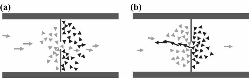
Figure 6: Alternating pedestrian flows at a bottleneck. These oscillations are self-organized and occur due to a pressure difference between the waiting crowd on one side and the crowd on the other side passing the bottleneck [after Helbing and Molnár (1995), Helbing (1997)].

Oscillations are a organization pattern of conflicting flows which allows to optimize the overall throughput under certain conditions (see Sec. 4.1). In pedestrian flows (see Fig. 6), the mechanism behind the self-induced oscillations is as follows: Pressure builds up on that side of the bottleneck where more and more pedestrians have to wait, while it is reduced on the side where pedestrians can move ahead and pass the bottleneck. If the pressure on one side exceeds the pressure on the other side by a certain amount, the passing direction is changed.

Transferring this self-organization principle to urban vehicle traffic, we define red and green phases in a way that considers “pressures” on the traffic light by road sections waiting to be served and “counter-pressures” from the subsequent road sections depending on the degree of congestion on them. Generally speaking, these pressures depend on delay times, queue lengths, or potentially other quantities as well. The proposed control principle is self-organized, autonomous, and adaptive to the respective local traffic situation, as will be shown below.

4.3 Basic switching rules for traffic lights

Our switching rules for traffic lights will have to solve the following control problems:

• The number of vehicles on a road section served by a green time period should be proportional to the average arrival flows $\overline{Q_{i}^{\rm arr}}$, at least if these are small.

• In order to avoid time losses due to yellow lights, switching of traffic lights should be minimized under saturated traffic conditions. However, single vehicles and small queues need to be served as well after some maximum cycle time $T^{\rm max}$.

• Despite of the desire to maintain green lights as long as possible, signal control should be able to react to changing traffic conditions in a flexible way. Unfortunately, the change of traffic conditions depends on traffic light control itself, so that a reliable forecast is only possible over short time periods.

• Under suitable conditions, traffic lights should synchronize themselves to establish green waves.

The synchronization of traffic lights is not only a matter of the adjustment of green and red time periods, i.e. of the frequency of control cycles: The adaptation of the time offset is also crucial for the establishment of green waves. While the adaptation problem is easily solvable for Manhattan-like road networks, the situation for irregular road networks is much more complex. Green waves may, in fact, cause major obstructions of crossing flows. Therefore, it is a great difficulty to find suitable rules which flows to prioritize. While addressing these points in the next paragraphs, we will develop a suitable control approach step by step. The resulting control principles may be also used to resolve conflicts between competing flows in other complex systems like production networks [Helbing (2003a, 2004, 2005), Helbing et al. (2004)], see Sec. 5.1.2.

The philosophy of our traffic light control is the minimization of the cumulative or average travel time and, therefore, of the cumulative delay time. Minimizing the overall delay time means to serve as many vehicles by the traffic lights as possible, i.e. to maximize the average departure rate (the average throughput). Let us explain this principle in more detail: If the traffic light is red or yellow, we have $\gamma_{i}(t)=0$ and the overall departure rate is $I_{i}Q_{i}^{\rm dep}(t)=0$. Otherwise, if the traffic light is green ($\gamma_{i}(t)=1$), we find

$$I_{i}Q_{i}^{\rm dep}(t)=\left\{\begin{array}[]{ll}I_{i}Q_{i}^{\rm arr}(t-L_{i}/V_{i}^{0})&\mbox{if }l_{i}(t)=0\,,\\ \min_{j}[I_{j}Q_{j}^{\rm dep}(t-L_{i}/|c|)/\alpha_{ij}]&\mbox{if }l_{j}(t)=L_{j}\,,\\ I_{i}Q_{i}^{\rm max}&\mbox{otherwise.}\end{array}\right.$$ (39)

A green light should be provided for the road section whose vehicle flow during a certain future time period is expected to be highest, taking into account any yellow-light related time losses. This principle tends to serve the road with the largest outflow, i.e. the largest number $I_{i}$ of lanes (see the third condition). However, it matters how long the maximum flow can be maintained, i.e. how large the number number $I_{i}l_{i}\rho^{\rm jam}$ of queued vehicles is. Moreover, vehicles in road section $i$ will be hardly able to depart (see the second condition), if one of the subsequent road sections $j$ is completely congested by the expected number $I_{i}Q_{i}^{\rm max}\alpha_{ij}(t-t^{\prime}_{0})$ of vehicles arriving between time $t^{\prime}_{0}$ and $t$. That is, a green light starting at time $t^{\prime}_{0}$ would usually end when the condition

$$I_{i}Q_{i}^{\rm max}(t-t^{\prime}_{0})\alpha_{ij}=I_{j}[L_{j}-l_{j}(t^{\prime}_{0})]\rho^{\rm jam}$$ (40)

is valid for the first time. Freely moving vehicles (see the first conditions) will have an impact comparable to the reduction of a queue (third condition) only, if

$$\frac{1}{t-t_{0}}\int\limits_{t_{0}}^{t}dt^{\prime}\;Q_{i}^{\rm arr}(t-L_{i}/V_{i}^{0})=\frac{N_{i}^{\rm arr}(t-L_{i}/V_{i}^{0})-N_{i}^{\rm arr}(t_{0}-L_{i}/V_{i}^{0})}{t-t_{0}}$$ (41)

is of the order $Q_{i}^{\rm max}$, where

$$N_{i}^{\rm arr}(t-L_{i}/V_{i}^{0})=\int\limits_{0}^{t}dt^{\prime}\;Q_{i}^{\rm arr}(t^{\prime}-L_{i}/V_{i}^{0})\,.$$ (42)

Summarizing this, the expected number $\Delta N_{i}^{\rm exp}$ of vehicles served before interruption by a red light at time $t_{1}$ can be often estimated by the cascaded minimum function

$$\Delta N_{i}^{\rm exp} = I_{i}Q_{i}^{\rm max}\,(t_{1}-t^{\prime}_{0})$$ (43)

$$= \rho^{\rm jam}\min\bigg{[}\!\underbrace{I_{i}l_{i}(t^{\prime}_{0})}_{\rm pressure}\,,\underbrace{\min_{j}\bigg{(}\frac{I_{j}[L_{j}-l_{j}(t^{\prime}_{0})]}{\alpha_{ij}}\bigg{)}}_{\rm counter-pressure}\!\bigg{]}\,,$$

where $t_{1}-t^{\prime}_{0}$ denotes the expected green time. However, generalizations of this formula are needed for the treatment of low traffic (see Sec. 4.5) and green waves (see Sec. 4.6).

As our control philosophy requires to reduce queues as fast as possible, the decision to serve a certain road section $i$ should be based on the greatest value of $\sum\Delta N_{i}^{\rm exp}/(t_{1}-t^{\prime}_{0})$, where the sum extends over all flows compatible with $Q_{i}^{\rm dep}$. If a switching time $\tau$ is necessary, the relevant formula is $\sum\Delta N_{i}^{\rm exp}/(t_{1}-t^{\prime}_{0}+\tau)$, instead. The switching decision should be regularly revised (e.g. every time period $\tau$), as the traffic situation may change.

Note that formula (43) implies that, given an equal number of lanes, green times are more likely for long queues, which could be said to exert some “pressure” on the traffic light. However, if road sections $j$ demanded by turning flows are congested, this exerts some “counter-pressure”. This will suppress green lights in cases where they would not allow to serve vehicles, i.e. where they would not make sense. As a consequence, while cycle times increase with growing arrival rates as long as these can be served, they may go down again when the road network is too congested.

4.4 Oscillations at a merge bottleneck

For the purpose of illustration, let us discuss a merge bottleneck (see Fig. 8). The two merging road sections $i\in\{1,2\}$ shall have the overall capacities $I_{i}Q^{\rm max}$ with $I_{1}\geq I_{2}$, while the subsequent section $j$ shall have the capacity $I_{j}Q^{\rm max}\geq I_{1}Q^{\rm max}$, so that no congestion will occur in the subsequent road section. Let us assume that the arrival flows $Q_{i}^{\rm arr}$ are constant in time. Furthermore, let us assume that the traffic light for road section 2 turns red at times $t_{0}$, $t_{2}$, etc., while the red lights for road section 1 start at $t_{1}$, $t_{3}$, etc. The green times for road section 1 begin after an yellow time period of $\tau$, i.e. at times $t^{\prime}_{2k}=t_{2k}+\tau$ and last for the time periods $t_{2k+1}-t^{\prime}_{2k}$.

We can distinguish the following cases:

• Equivalent road sections: If $I_{1}=I_{2}$, the queues on both road sections will be completely cleared in an alternating way, see Fig. 7(a). In case of growing vehicle queues, the green times grow accordingly.

• One main and one side road ($I_{1}>I_{2}$):

  • If the arrival flow $Q_{2}^{\rm arr}$ of road section 2 (the side road) is low, both roads are completely cleared.

  • In many cases, however, the queue length in the side road grows in the course of time, while the queue in the main road (road section 1) is completely cleared, see Fig. 7(b). As a consequence, road section 2 will be fully congested after some time period, which limits a further growth of the queue and discourages drivers to use this road section according to our traffic assignment rule. In extreme cases, when no maximum cycle time is implemented (see Sec. 4.4.3), the main road may have a green light all the time, while road section 2 (the side road) is never served, see Fig. 7(c).

  • If the sum $\sum_{i}I_{i}Q_{i}^{\rm arr}$ of overall arrival flows exceeds the capacity $I_{j}Q^{\rm max}$ of the subsequent road section $j$, the queue on both road sections will grow, see Fig. 7(d).

We will now discuss these cases in more detail.

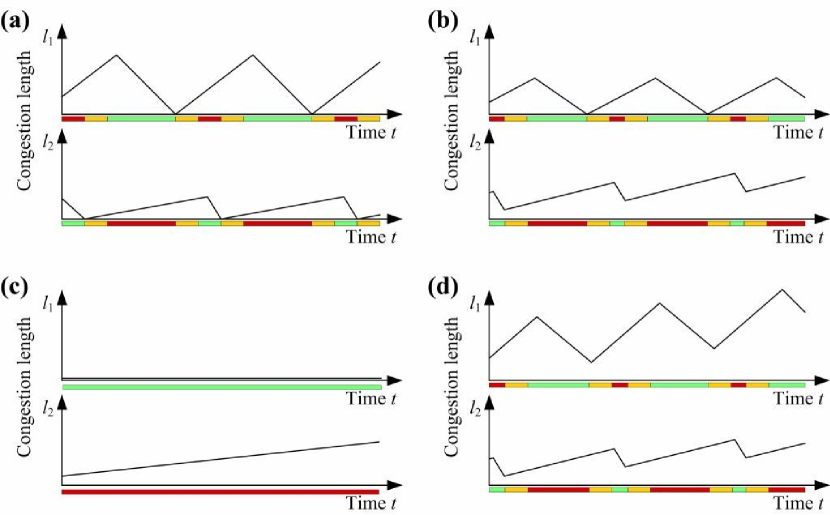
Figure 7: Different cases of the self-organized control of a merge bottleneck: (a) The vehicle queue in each road section is completely cleared, before the traffic light turns red. (b) The traffic light in the side road turns red, before the vehicle queue has fully disappeared, but the main road is fully cleared. (c) In extreme cases, if a maximum cycle time is not enforced, the side road would never get a green light and the main road would always be served. (d) When the sum of arrival rates is higher than the capacity of the subsequent road section, the vehicle queues in both road sections may grow under certain conditions (see text).

4.4.1 Equivalent road sections

Let us assume the queue length on road section 2 is zero at time $t_{0}$ and the traffic light switches to red in order to offer a green light to road section 1 at time $t^{\prime}_{0}=t_{0}+\tau$. The queue length at time $t$ is given by

$$l_{1}(t)=l_{1}(t^{\prime}_{0})+C_{1}(t-t^{\prime}_{0})\,,$$ (44)

where

$$C_{i}=\left(\frac{\rho^{\rm jam}}{Q_{i}^{\rm arr}}-\frac{1}{V_{i}^{0}}\right)^{-1}=\frac{Q_{i}^{\rm arr}}{\rho^{\rm jam}-Q_{i}^{\rm arr}/V_{i}^{0}}$$ (45)

according to Eq. (8). Note that, in the limit of small arrival rates $Q_{i}^{\rm arr}$, this queue expansion velocity is proportional to $Q_{i}^{\rm arr}$. The reduction of the queue starts with the green phase and is proportional to $c$. We, therefore, have the following equation for the length of the effective queue (= queue length minus area of quasi-free traffic):

$$l_{1}^{\rm eff}(t)=l_{1}(t)+c(t-t^{\prime}_{0})=l_{1}(t^{\prime}_{0})+C_{1}(t-t^{\prime}_{0})-|c|(t-t^{\prime}_{0})\,.$$ (46)

The effective queue length disappears at time

$$t_{0}^{*}=t^{\prime}_{0}+\frac{l_{1}(t^{\prime}_{0})}{|c|-C_{1}}\,.$$ (47)

However, the last vehicle of the queue needs an additional time period of $l_{1}(t_{0}^{*})/V_{1}^{0}$ to leave the road section, so that the queue length $l_{1}(t)$ in road section 1 becomes zero at time $t=t_{1}$ with

$$t_{1}=t_{0}^{*}+\frac{l_{1}(t_{0}^{*})}{V_{1}^{0}}=\dots=t^{\prime}_{0}+l_{1}(t^{\prime}_{0})\frac{1+|c|/V_{1}^{0}}{|c|-C_{1}}\,.$$ (48)

At that time, the traffic light for road section 1 switches to red and road section 2 is served by a green light starting at $t^{\prime}_{1}=t_{1}+\tau$. Analogous considerations show that the queue in road section 2 is cleared at time

$$t_{2}=t^{\prime}_{1}+l_{2}(t^{\prime}_{1})\frac{1+|c|/V_{2}^{0}}{|c|-C_{2}}\,.$$ (49)

The next green time for road section 1 starts at time $t^{\prime}_{2}=t_{2}+\tau$ and ends at

$$t_{3}=t^{\prime}_{2}+l_{1}(t^{\prime}_{2})\frac{1+|c|/V_{1}^{0}}{|c|-C_{1}}\,.$$ (50)

We can determine the queue length $l_{1}(t^{\prime}_{2})$ at the beginning of the green phase as the queue length that has built up during the previous red phase of length $t_{2}-t^{\prime}_{1}$ and two yellow phases of duration $\tau$ each. As a consequence, we find $l_{1}(t^{\prime}_{2})=C_{1}(t_{2}-t^{\prime}_{1}+2\tau)$. In the stationary case we have $l_{1}(t^{\prime}_{2})=l_{1}(t^{\prime}_{0})$ and $l_{1}(t_{1})=0$, as the queue on road section 1 is completely cleared at time $t_{1}$. This eventually leads to a rather complicated formula for $t_{2}-t^{\prime}_{1}$, which is proportional to the respective queue length. For small values of the arrival rates $Q_{i}^{\rm arr}$, one can show that the green times are proportional to $C_{i}$ and $Q_{i}^{\rm arr}$. That is, the duration of the green phases is proportional to the arrival rates, as expected, if the arrival rates are small enough. The cycle time grows linearly with $Q_{1}^{\rm arr}+Q_{2}^{\rm arr}$.

4.4.2 One main and one side road

If both road sections are completely cleared as in case (i) above, the mathematical treatment is analogous to the previous section. More interesting is case (ii), in which the traffic light for road section 2 switches to red already before the queue is cleared completely, see Fig. 7(b). While Eqs. (48) and (50) are still valid, we have to find other expressions for $t_{2}$ and $l_{1}(t^{\prime}_{2})=l_{1}(t^{\prime}_{0})$. Let $t_{2}^{+}$ be the time point in which the queue of length $l_{1}(t_{2})$ in road section 1 at time $t_{2}$ would be completely resolved, if the traffic light would turn green for road section 1 at time $t_{2}$. Road section $1$ could for sure deliver an overall flow of $I_{1}Q^{\rm max}$ between $t^{\prime}_{2}=t_{2}+\tau$ and $t_{2}^{+}$, while the departure flow from road section 1 could be much smaller than $I_{1}Q^{\rm max}$ afterwards. In order to switch to green in favor of road section 1, it is, therefore, reasonable to demand

$$I_{1}Q^{\rm max}[t_{2}^{+}-(t_{2}+\tau)]\geq I_{2}Q^{\rm max}(t_{2}^{+}-t_{2})\,.$$ (51)

This formula considers the time loss $\tau$ by switching due to the intermediate yellow period, and it presupposes that $Q^{\rm max}(t_{2}^{+}-t_{2})\geq l_{2}(t_{2})\rho^{\rm jam}$, i.e. road section 2 can maintain the maximum flow $Q^{\rm max}$ until $t_{2}^{+}$. Our philosophy is to give a green light to the road section which can serve most vehicles during the next time period $t_{2}^{+}-t_{2}$. The equation to determine $t_{2}^{+}=t_{2}^{-}+l_{1}(t_{2})/V_{1}^{0}$ is $l_{1}(t_{2})=|c|[t_{2}^{-}-(t_{2}+\tau)]$ with $l_{1}(t_{2})=C_{1}(t_{2}-t_{1})$. This leads to $t_{2}^{-}=t_{2}+\tau+C_{1}(t_{2}-t_{1})/|c|$ and

$$t_{2}^{+}=(t_{2}+\tau)+\left(\frac{C_{1}}{|c|}+\frac{C_{1}}{V_{1}^{0}}\right)(t_{2}-t_{1})\,,$$ (52)

while Eq. (51) implies

$$t_{2}^{+}-t_{2}\geq\frac{\tau}{1-I_{2}/I_{1}}\,.$$ (53)

Together with Eq. (52) we find

$$t_{2}-t_{1}=\left.\frac{\tau}{I_{1}/I_{2}-1}\right/\!\left(\frac{C_{1}}{|c|}+\frac{C_{1}}{V_{1}^{0}}\right)\,.$$ (54)

For $I_{1}=I_{2}$, one can immediately see that the traffic light would never switch before the queue in road section 2 is fully resolved. However, early switching could occur for $I_{1}>I_{2}$.

Once the traffic light is turned green at time $t_{2}$, the vehicles which have queued up until time $t_{2}^{+}$ will be served with the overall rate $I_{1}Q^{\rm max}$ as well, until the departure flow is given by the lower arrival flow $Q_{1}^{\rm arr}$ at time $t_{3}$ and later. The time point $t_{2}^{*}$ at which the effective queue resolves is given by $l_{1}(t_{2}^{*})=|c|[t_{2}^{*}-(t_{2}+\tau)]$, which results in

$$t_{2}^{*}-t_{2}=\frac{t_{2}^{-}-t_{2}}{1-C_{1}/|c|}=\frac{\tau+C_{1}(t_{2}-t_{1})/|c|}{1-C_{1}/|c|}\,.$$ (55)

The last vehicle of the queue has left road section 1 at time $t_{3}$ with

$$t_{3}-t_{2}=\frac{t_{2}^{+}-t_{2}}{1-C_{1}/|c|}=\frac{\tau}{(1-I_{2}/I_{1})(1-C_{1}/|c|)}\,.$$ (56)

Afterwards, the overall departure flow drops indeed to $I_{1}Q_{1}^{\rm arr}$, and the traffic light tends to turn red if $I_{1}Q_{1}^{\rm arr}<I_{2}Q^{\rm max}$. Otherwise, it will continue to stay green during the whole rush hour. Considering $l_{1}(t_{3})=0=l_{1}(t_{1})$ and $l_{1}(t^{\prime}_{2})=C_{1}(t^{\prime}_{2}-t_{1})$, one can determine all quantities. One can show that the green time fraction for road section 1 grows proportionally to $Q_{1}^{\rm arr}$, if $\tau$ is small. Moreover, one can derive that the green time fractions of both road sections and the cycle time $T^{\rm cyc}=t_{3}-t_{1}$ are proportional to $C_{1}$, i.e. the main road dominates the dynamics. The queue length on road section 2 tends to grow, as it is never fully cleared.

If $I_{1}Q_{1}^{\rm arr}+I_{2}Q_{2}^{\rm arr}>I_{j}Q^{\rm max}$, it can also happen that the queues grow in both road sections. This is actually the case, if $I_{1}Q_{1}^{\rm arr}>I_{j}Q^{\rm max}$, see Fig. 7(d). Moreover, in the case $I_{2}Q^{\rm max}<I_{1}Q_{1}^{\rm arr}$, road section 2 would never be served, see Fig. 7(c). This calls for one of several possible solutions: 1. Allow turning on red. 2. Decide to transform the side road into a dead end. 3. Build a bridge or tunnel. 4. Use roundabouts or other road network designs which do not require traffic lights. 5. Treat main and side roads equivalently, i.e. set $I_{1}=I_{2}=1$ in the above formulas, or specify suitable parameter values for $I_{i}$, although it will increase the overall delay times. 6. Restrict the red times to a maximum value at the cost of increased overall delay times and reduced intersection throughput.

4.4.3 Restricting red times

In order to avoid excessive cycle times, one has to set upper bounds. This may be done as follows: Let $T^{\rm max}$ be the maximum allowed cycle time,

$$\overline{\gamma_{i}}=\frac{1}{T^{\rm max}}\!\!\!\int\limits_{t-T^{\rm max}}^{t}\!\!\!dt^{\prime}\;\gamma_{i}(t^{\prime})$$ (57)

the green time fraction within this time interval, and

$$\overline{Q_{i}^{\rm arr}}=\frac{1}{T^{\rm max}}\!\!\!\int\limits_{t-T^{\rm max}}^{t}\!\!\!dt^{\prime}\;Q_{i}^{\rm arr}(t^{\prime})$$ (58)

the average arrival rate. If $\overline{\gamma_{i}}$ exceeds a specified green time fraction $u_{i}^{0}$, the green light will be switched to red. This approach also solves the problem that even small vehicle queues or single vehicles must be served within some maximum time period.

The green time fractions $u_{i}^{0}$ may slowly vary in time and could be specified proportionally to the relative arrival rate $\overline{Q_{i}^{\rm arr}}/\sum_{i^{\prime}}\overline{Q_{i^{\prime}}^{\rm arr}}$, with some correction for the yellow time periods. However, it is better to determine the green time fractions $u_{i}^{0}$ in a way that helps to optimize the system performance (see Sec. 5.1.1).

4.4.4 Intersection capacity and throughput

Let us finally calculate the average throughput $Q^{\rm all}$ of the signalized intersection. When the traffic volume is low, it is determined by the sum $\sum_{i}I_{i}\overline{Q_{i}^{\rm arr}}$ of average arrival flows, while at high traffic volumes, it is given by the intersection capacity

$$Q^{\rm cap}=Q^{\rm max}\frac{I_{1}(t_{3}-t^{\prime}_{2})+I_{2}(t_{2}-t^{\prime}_{1})}{t_{3}-t_{1}}=Q^{\rm max}\frac{I_{1}(t_{3}-t^{\prime}_{2})+I_{2}(t_{2}-t^{\prime}_{1})}{T^{\rm cyc}}\,.$$ (59)

This implies

$$Q^{\rm all}=\min\left(\sum_{i}I_{i}\overline{Q_{i}^{\rm arr}},Q^{\rm cap}\right)\,.$$ (60)

According to these formulas, the losses in throughput and capacity by the yellow times $2\tau$ are reduced by longer green times $t_{3}-t^{\prime}_{2}$ and $t_{2}-t^{\prime}_{1}$. Our calculations indicate that our switching rule automatically increases the cycle time $T^{\rm cyc}=t_{3}-t_{1}$ and the intersection capacity $Q^{\rm cap}$, when the arrival rates $Q_{i}^{\rm arr}$ of equivalent roads with $I_{1}=I_{2}$ or the arrival rate $Q_{1}^{\rm arr}$ of a main road are increased. Figure 8 shows the cycle time $T^{\rm cyc}$, throughput $Q^{\rm all}$, and green time fraction $u_{1}$ as a function of $Q_{i}^{\rm arr}=Q^{\rm arr}$ for different values of $I_{1}/I_{2}$.

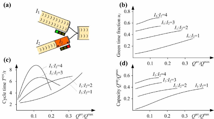
Figure 8: (a) Illustration of the traffic control of a merge bottleneck for constant arrival rates and a non-congested outflow. The characteristic behavior of the proposed self-organized traffic light control depends on the number $I_{i}$ of lanes of the entering road sections $i$ and on the arrival rates $Q_{i}^{\rm arr}$: (b) Actual green time fraction $u_{1}$ for $Q_{2}^{\rm arr}=\mbox{const.}$ and variable $Q_{1}^{\rm arr}$, (c) cycle time $T^{\rm cyc}$ as compared to the yellow time period $\tau$ for $Q_{2}^{\rm arr}=Q_{1}^{\rm arr}$, and (d) actual throughput $Q^{\rm all}$ of the signalized intersection in comparison with the maximum uninterrupted flow $Q^{\rm max}$ per lane for $Q_{2}^{\rm arr}=Q_{1}^{\rm arr}$.

4.5 Serving single vehicles at low traffic volumes

While traffic lights have been invented to efficiently coordinate and serve vehicle flows at high traffic volumes, they should ideally provide a green light for every arriving vehicle at low average arrival rates $\overline{Q}_{i}^{\rm arr}$. According to formula (39), the departure flow $Q_{i}^{\rm dep}(t)$ will, in fact, be 0 most of the time on all road sections. Only during short time periods, single vehicles will randomly cause positive values of $Q_{i}^{\rm arr}(t-L_{i}/V_{i}^{0})$ on one of the road sections $i$. The traffic light should be turned green shortly before the arrival of the vehicle at the downstream boundary of this road section. If switching requires a time period of $\tau$, the arrival flow $Q_{i}^{\rm arr}(t-L_{i}/V_{i}^{0}+\tau)$ would need to trigger a switching of the traffic light in favor of road section $i$. Considering this and formula (39), it is essential to take a switching decision based on the departure flow $Q_{i}^{\rm dep}(t+\tau)$ expected at time $t+\tau$. The departure flow $Q_{i}^{\rm dep}(t)$ can, in fact, be forecasted for a certain time period based on available flow data and assumed states of neighboring signals. In order to minimize the time period $\tau$, it makes sense to switch any traffic light to red, if no other vehicle is following. That is, at low traffic volumes, all traffic lights would be red most of the time. However, any single vehicle would trigger an anticipative green light upon arrival, so that vehicles would basically never have to wait at a red light.

4.6 Emergence of green waves through self-organized synchronization

In order to let green waves emerge in a self-organized way, the control strategy must show a tendency to form vehicle groups, i.e. convoys, and to serve them just as they approach an intersection. For this to happen, small vehicle clusters must potentially be delayed, which gives them a chance to grow. When they are released, the corresponding “convoys” may themselves trigger a green wave.

In fact, the ideal situation would be that traffic flow from road section $i$ arrives at location $L_{j}-l_{j}(t)$ in a subsequent road section $j$ just when the effective queue $l_{j}^{\rm eff}(t)$ has resolved. This is equivalent with the need to arrive at location $L_{j}$ just at the moment when the queue length $l_{j}(t)$ becomes zero. Under such conditions, free arrival flows $Q_{j}^{\rm arr}(t-L_{j}/V_{j}^{0})$ with values around $Q_{i}^{\rm max}$ would immediately follow the high outflow $Q_{j}^{\rm dep}=Q_{j}^{\rm max}$ from the (resolving) congested area in road section $j$ (here, we assume $I_{i}=I_{j}$). As a consequence, the green light at the end of road section $j$ would be likely to continue. This mechanism could establish a synchronization among traffic lights, i.e. a green wave by suitable adjustment of the time offsets, triggered by vehicle flows. As it requires a time period $\Delta t_{j}=[L_{j}-l_{j}(t)]/V_{j}^{0}$ to reach the upstream congestion front in section $j$, it will be required to turn the signal of the previous road section $i$ green a time period $\Delta t_{j}$ before the effective queue is expected to resolve. This time period defines the necessary forecast time interval.

When the effective queue of length $l_{j}^{\rm eff}(t)$ is resolved, the related sudden increase in $L_{j}-l_{j}(t)$ can cause a sudden increase in $\Delta N_{i}^{\rm pot}$ and, thereby, possibly trigger a switching of the traffic light. The emergence of green waves obviously requires that the green light at the end of road section $j$ should stay long enough to resolve the queue. This is likely, if road section $j$ is a main road (arterial), see our considerations in Sec. 4.4.2.

In a more abstract sense, the intersections in the road network can be understood as self-sustained oscillators which are coupled by the vehicle flows between them. Therefore, one might expect them to synchronize like many natural systems do [Pikovsky et al. (2001)]. Interestingly, even if the intersections are not coupled artificially with some communication feedback, the weak coupling via vehicle flows is sufficient to let larger areas of the road network synchronize. The serving direction percolates through the network, stabilizes itself for a while and is then taken over by another serving direction. In other words, neighboring intersections affect each other by interactions via vehicle flows, which favors a mutual adjustment of their rhythms. This intrinsic mechanism introduces order, so that vehicle flows are coordinated.

5 Summary and outlook

In this contribution, we have presented a section-based traffic model for the simulation and analysis of network traffic. Moreover, we have proposed a decentralized control strategy for traffic flows, which has certain interesting features: Single arriving vehicles always get a green light. When the intersection is busy, vehicles are clustered, resulting in an oscillatory and efficient service (even of intersecting main flows). If possible, vehicles are kept going in order to avoid capacity losses produced by stopped vehicles. This principle bundles flows, thereby generating main flows (arterials) and subordinate flows (side roads and residential areas). If a road section cannot be used due to a building site or an accident, traffic flexibly re-organizes itself. The same applies to different demand patterns in cases of mass events, evacuation scenarios, etc. Finally, a local dysfunction of sensors or control elements can be handled and does not affect the overall system. A large-scale harmonization of traffic lights is reached by a feedback between neighboring traffic lights based on the vehicle flows themselves, which can synchronize traffic signals and organize green waves. In summary, the system is self-organized based on local information, local interactions, and local processing, i.e. decentralized control. However, a multi-hierarchical feedback may further enhance system performance by increasing the speed of large-scale information exchange and the speed of synchronization in the system.

We should point out some interesting differences compared to conventional traffic control:

• The green phases of a traffic light depend on the respective traffic situation on the previous and the subsequent road sections. They are basically determined by actual and expected queue lengths and delay times. If no more vehicles need to be served or one of the subsequent road sections is full, green times for one direction will be terminated in favor of green times for other directions. The default setting corresponds to red lights, as this enables one to respond quickly to approaching traffic. Therefore, during light traffic conditions, single vehicles can trigger a green light upon arrival at the traffic signal.

• Our approach does not use precalculated or predetermined signal plans. It is rather based on self-organized red and green phases. In particularly, there is no fixed cycle time or a given order of green phases. Some roads may be even served more frequently than others. For example, at very low traffic volumes it can make sense to serve the same road again before all other road sections have been served. In other words, traffic optimization is not just a matter of green times and their permutation.

• Instead of a traffic control center, we suggest a distributed, local control in favor of greater flexibility and robustness. The required information can be gathered by optical or infrared sensors, which will be cheaply available in the future. Complementary information can be obtained by a coupling with simulation models. Apart from the section-based model proposed in this paper, one can also use other (e.g. microsimulation) models with or without stochasticity, as our control approach does not depend on the traffic model. Travel time information to enhance route choice decisions may be transmitted by mobile communication.

• Pedestrians could be detected by modern sensors as well and handled as additional traffic streams. Alternatively, they may get green times during compatible green phases for vehicles or after the maximum cycle time $T^{\rm max}$. Public transport (e.g. busses or trams) may be treated as vehicles with a higher weight. A natural choice for the weight would be the average number of passengers. This would tend to prioritize public transport and to give it a green light upon arrival at an intersection. In fact, a prioritization of public transport harmonizes much better with our self-organized traffic control concept than with precalculated signal plans.

5.1 Future research directions

5.1.1 Towards the system optimum

Traffic flow optimization in networks is not just a matter of durations, frequencies, time offsets and the order of green times, which may be adjusted in the way described above. Conflicts of flows and related inefficiencies can also be a result of the following problems:

• Space which is urgently required for certain origin-destination flows may be blocked by other flows, causing a spill-over and blockage of upstream road sections. One of the reasons for this is the cascaded minimum function (25). It may, therefore, be helpful to restrict turning only to subsequent road sections that are normally not fully congested (i.e. wide and/or long road sections).

• Giving green times to compatible vehicle flows may cause the over-proportional service of certain road sections. These over-proportional flows may be called parasitic. They may cause the blockage of space in subsequent road sections which would be needed for other flow directions. In order to avoid parasitic flows, it may be useful to restrict the green times of compatible flow directions.

• Due to the selfish route choice behavior, drivers tend to distribute over alternative routes in a way that establishes a Wardrop equilibrium (also called a Nash or user equilibrium) [Papageorgiou (1991)]. This reflects the tendency of humans to balance travel times [Helbing et al. (2002)]. That is, all subsequent road sections $j$ of $i$ used to reach a destination $d$ are characterized by (more or less) equal travel times. If the travel time on one path was less than on alternative ones, more vehicles would choose it, which would cause more congestion and a corresponding increase in travel times.

In order to reach the system optimum, which is typically defined by the minimum of the overall travel times, the drivers have to be coordinated. This would be able to further enhance the capacity of the traffic network, but it would require the local adaptation of signal control parameters. For example, the enforcement of optimal green time fractions $u_{i}^{0}$ based on the method described in Sec. 4.4.3 would be one step into this direction, as it is not necessarily the best, when green time fractions are specified proportionally to the arrival rates $Q_{i}^{\rm arr}$.

Unfortunately, green time fractions $u_{i}^{0}$ do not allow to differentiate between different origin-destination flows using the same road section. Such a differentiation would allow one to reserve certain capacities (i.e. certain fractions of road sections) for specific flows. This could be reached by advanced traveller information systems (ATIS) [Hu and Mahmassani (1997), Mahmassani and Jou (2000), Schreckenberg and Selten (2004)] together with suitable pricing schemes, which would increase the attractiveness of some routes compared to others.

Different road pricing schemes have been proposed, each of which has its own advantages and disadvantages or side effects. Congestion charges, for example, could discourage to take congested routes required to reach minimum average travel times, while conventional tolls and road pricing may reduce the trip frequency due to budget constraints (which potentially interferes with economic growth and fair chances for everyone’s mobility).

In order to activate capacity reserves, we therefore propose an automated route guidance system based on the following principles: After specification of their destination, drivers should get individual route choice recommendations in agreement with the traffic situation and the route choice proportions required to reach the system optimum. If an individual selects a faster route instead of the recommeded route it should, on the one hand, have to pay an amount proportional to the increase in the overall travel time compared to the system optimum. On the other hand, drivers not in a hurry should be encouraged to take the slower route $i$ by receiving the amount of money corresponding to the related decrease in travel times. Altogether, such an ATIS could support the system optimum while allowing for some flexibility in route choice. Moreover, the fair usage pattern would be cost-neutral for everyone, i.e. traffic flows of potential economic relevance would not be suppressed by extra costs.

5.1.2 On-line production scheduling

Our approach to self-organized traffic light control could be also transfered to a flexible production scheduling, in order to cope with problems of multi-goal optimization, with machine breakdowns, and variations in the consumption rate. This could, for example, help to optimize the difficult problem of re-entrant production in the semiconductor industry [Beaumariage and Kempf (1994), Diaz-Rivera et al. (2000), Helbing (2005)].

In fact, the control of network traffic flows shares many features with the optimization of production processes. For example, travel times correspond to cycle times, cars with different origins and destinations to different products, traffic lights to production machines, road sections to buffers. Moreover, variations in traffic flows correspond to variations in the consumption rate, congested roads to full buffers, accidents to machine breakdowns, and conflicting flows at intersections to conflicting goals in production management. Finally, the cascaded minimum function (25) reflects the fact that the scarcest resource governs the maximum production speed: If a specific required part is missing, a product cannot be completed. All of this underlines the large degree of similarity between traffic and production networks [Helbing (2005)]. As a consequence, one can apply similar methods of description and similar control approaches.

99

References

- [Beaumariage and Kempf (1994)] Beaumariage, T., and Kempf, K. The nature and origin of chaos in manufacturing systems. In: Proceedings of 1994 IEEE/SEMI Advanced Semiconductor Manufacturing Conference and Workshop, pp. 169–174, Cambridge, MA, 1994.
- [Ben-Akiva, McFadden et al. (1999)] Ben-Akiva, M., McFadden, D. M. et al. Extended framework for modeling choice behavior. Marketing Letters, 10:187–203, 1999.
- [Brockfeld et al. (2001)] Brockfeld, E., Barlovic, R., Schadschneider, A., and Schreckenberg, M. Optimizing traffic lights in a cellular automaton model for city traffic. Physical Review E, 64:056132, 2001.
- [Chrobok et al. (2000)] Chrobok, R., Kaumann, O., Wahle, J., and Schreckenberg, M. Three categories of traffic data: Historical, current, and predictive. In: E. Schnieder and U. Becker (eds), Proceedings of the 9th IFAC Symposium ‘Control in Transportation Systems’, pp. 250–255, Braunschweig, 2000.
- [Cremer and Ludwig (1986)] Cremer, M., and Ludwig, J. A fast simulation model for traffic flow on the basis of Boolean operations. Mathematics and Computers in Simulation, 28:297–303, 1986.
- [Daganzo (1995)] Daganzo, C. The cell transmission model, Part II: Network traffic. Transportation Research B, 29:79–93, 1995.
- [Diakaki et al. (2003)] Diakaki, C., Dinopoulou, V., Aboudolas, K., Papageorgiou, M., Ben-Shabat, E., Seider, E., and Leibov, A. Extensions and new applications of the traffic signal control strategy TUC. Transportation Research Board, 1856:202-211, 2003.
- [Diaz-Rivera et al. (2000)] Diaz-Rivera, I., Armbruster, D., and Taylor, T. Periodic orbits in a class of re-entrant manufacturing systems. Mathematics and Operations Research, 25:708–725, 2000.
- [Elloumi et al. (1994)] Elloumi, N., Haj-Salem, H., and Papageorgiou, M. METACOR: A macroscopic modelling tool for urban corridors. TRISTAN II (Triennal Symposium on Transportation Analysis), 1:135–150, 1994.
- [Esser and Schreckenberg (1997)] Esser, J., and Schreckenberg, M. Microscopic simulation of urban traffic based on cellular automata. International Journal of Modern Physics C, 8(5):1025, 1997.
- [Fouladvand and Nematollahi (2001)] Fouladvand, M. E., and Nematollahi, M. Optimization of green-times at an isolated urban crossroads. European Physical Journal B, 22:395–401, 2001.
- [Gartner (1990)] Gartner, N. H. OPAC: Strategy for demand-responsive decentralized traffic signal control. In: J.P. Perrin (ed), Control, Computers, Communications in Transportation, pp. 241–244, Oxford, UK, 1990.
- [Helbing (1997)] Helbing, D. Verkehrsdynamik [Traffic Dynamics]. Springer Verlag, 1997.
- [Helbing (2003a)] Helbing, D. Modelling supply networks and business cycles as unstable transport phenomena. New Journal of Physics, 5:90.1–90.28, 2003.
- [Helbing (2003b)] Helbing, D. A section-based queueing-theoretical traffic model for congestion and travel time analysis in networks. Journal of Physics A: Mathematical and General, 36:L593–L598, 2003.
- [Helbing (2004)] Helbing, D. Modeling and optimization of production processes: Lessons from traffic dynamics. In: G. Radons and R. Neugebauer (eds), Nonlinear Dynamics of Production Systems, pp. 85–105, Wiley, NY, 2004.
- [Helbing (2005)] Helbing, D. Production, supply, and traffic systems: A unified description. In: S. Hoogendoorn, P.V.L. Bovy, M. Schreckenberg, and D.E. Wolf (eds) Traffic and Granular Flow ’03, Berlin, 2005.
- [Helbing et al. (2004)] Helbing, D., Lämmer, S., Witt, U., and Brenner, T. Network-induced oscillatory behavior in material flow networks and irregular business cycles. Physical Review E, 70:056118, 2004.
- [Helbing and Molnár (1995)] Helbing, D., and Molnár, P. Social force model of pedestrian dynamics. Physical Review E, 51:4282–4286, 1995.
- [Helbing et al. (2002)] Helbing, D., Schönhof, M., and Kern, D. Volatile decision dynamics: Experiments, stochastic description, intermittency control, and traffic optimization. New Journal of Physics, 4:33.1–33.16, 2002.
- [Henry and Farges (1989)] Henry, J. J., and Farges, J. L. PRODYN. In: J.P. Perrin (ed), Control, Computers, Communications in Transportation, pp. 253–255, Oxford, UK, 1989.
- [Hu and Mahmassani (1997)] Hu, T.-Y., and Mahmassani, H. S. Day-to-day evolution of network flows under real-time information and reactive signal control. Transportation Research C, 5(1):51–69, 1997.
- [Huang and Huang (2003)] Huang, D.-W., and Huang, W.-N. Traffic signal synchronization. Physical Review E, 67:056124, 2003.
- [Lebacque (2005)] Lebacque, J. P. Intersection modeling, application to macroscopic network traffic flow modeling and traffic management. In: S. Hoogendoorn, P. H. L. Bovy, M. Schreckenberg, and D. E. Wolf (eds) Traffic and Granular Flow ’03, Springer, Berlin, 2005.
- [Li et al. (2004)] Li, Z., Wang, H., and Han, L.D. A proposed four-level fuzzy logic for traffic signal control. Transportation Research Board, CDROM Proceedings, 2004.
- [Lighthill and Whitham (1955)] Lighthill, M. J., and Whitham, G. B. On kinematic waves: II. A theory of traffic on long crowded roads. Proceedings of the Royal Society A, 229:317–345, 1955.
- [Lin and Chen (2004)] Lin, D., and Chen, R.L. Comparative evaluation of dynamic TRANSYT and SCATS based signal control logic using microscopic traffic simulations. Transportation Research Board, CDROM Proceedings, 2004.
- [Lotito et al. (2002)] Lotito, P., Mancinelli, E., and Quadrat J.P. MaxPlus Algebra and microscopic modelling of traffic systems. In: J.P. Lebacque, M. Rascle, and J.P. Quadrat (eds), Actes de l’Ecole d’Automne: Modélisation mathématique du traffic véhiculaire, Actes INRETS (in print), 2004.
- [Mahmassani and Jou (2000)] Mahmassani, H. S., and Jou, R. C. Transferring insights into commuter behavior dynamics from laboratory experiments to field surveys. Transportation Research A, 34:243–260, 2000.
- [Mancinelli et al. (2001)] Mancinelli, E., Cohen, G., Quadrat, J.P., Gaubert, S., and Rofman, E. On traffic light control of regular towns. INRIA Report 4276, 2001.
- [Mauro and Di Taranto (1989)] Mauro, V., and Di Taranto, C. UTOPIA. In: J.P. Perrin (ed), IFAC Control, Computers, Communications in Transportation, pp. 575-597, Paris, 1989.
- [Nagel et al. (2000)] Nagel, K., Esser, J., and Rickert M. Large-scale traffic simulations for transport planning. In: D. Stauffer (ed), Annual Review of Computational Physics VII, pp.151–202, World Scientific, 2000.
- [Niittymäki (2002)] Niittymäki, J. Fuzzy traffic signal control. In: M.Patriksson, M. Labbé (eds) Transportation Planning: State of the Art, Kluwer Academic Publishers, 2002.
- [Papageorgiou (1991)] Papageorgiou, M. Concise Encyclopedia of Traffic and Transportation Systems. Pergamon Press, 1991.
- [Pikovsky et al. (2001)] Pikovsky, A., Rosenblum, M., and Kurths, J. Synchronization. A Universal Concept in Nonlinear Sciences. Cambridge University Press, 2001.
- [Robertson (1997)] Robertson, D. The TRANSYT method of co-ordinating traffic signals. Traffic Engineering and Control, 76–77, 1997.
- [Robertson and Bretherton (1991)] Robertson, D., and Bretherton, R.D. Optimising networks of traffic signals in real-time: The SCOOT method. IEEE Transactions on Vehicular Technology, 40(1):11–15, 1991.
- [Sayers et al. (1998)] Sayers, T., Anderson, J., and Bell, M. Traffic control system optimization: a multiobjective approach. In: J.D. Grifiths (ed), Mathematics in Transportation Planning, Pergamon Press, 1998.
- [Scémama (1994)] Scémama, G. “CLAIRE”: a context free Artificial Intelligence based supervior for traffic control. In: M. Bielli, G. Ambrosino, and M. Boero (eds), Artificial Intelligence Applications to Traffic Engineering, pp. 137–156, Zeist, Netherlands, 1994.
- [Schreckenberg and Selten (2004)] Schreckenberg, M., and Selten, R. Human Behaviour and Traffic Networks. Springer Verlag, 2004.
- [Sims and Dobinson (1979)] Sims, A.G., and Dobinson, K.W. SCAT: the Sydney co-ordinated adaptative traffic system philosophy and benefits. Proceedings of the International Symposium on Traffic Control Systems, Volume 2B, pp. 19-41, 1979.
- [Stamatiadis and Gartner (1999)] Stamatiadis, C., and Gartner, N. Progression optimization in large urban networks: a heuristic decomposition approach. In: A. Ceder (ed), Transportation and Traffic Theory, pp. 645–662, Pergamon Press, 1999.
- [Stirn (2003)] Stirn, A. Das Geheimnis der grünen Welle [The secret of the green wave]. Süddeutsche Zeitung, June 17, 2003.
- [Treiber at al. (1999)] Treiber, M., Hennecke, A., and Helbing, D. Derivation, properties, and simulation of a gas-kinetic-based, non-local traffic model. Physical Review E, 59:239–253, 1999.