Analytical solution of the Thomas-Fermi equation for atoms

Abstract

An approximate analytical solution of the Thomas-Fermi equation for neutral atoms is obtained, using the Ritz variational method, which reproduces accurately the numerical solution, in the range $0\leq x\leq 50$, and its derivative at $x=0$. The proposed solution is used to calculate the total ionization energies of heavy atoms. The obtained results are in good agreement with the Hartree-Fock ones and better than those obtained from previously proposed trial functions by other authors.

I INTRODUCTION

Since the first works of Thomas and Fermi 1 , there have been many attempts to construct an approximate analytical solution of the Thomas-Fermi equation for atoms 1 . E.Roberts 2 suggested a one-parameter trial function:

$$\phi_{1}(x)=(1+\eta\sqrt{x})e^{-\eta\sqrt{x}},$$ (1)

where $\eta=1.905$ and Csavinsky 3 has proposed a two-parameters trial function:

$$\phi_{2}(x)=(a_{0}e^{-\alpha_{0}x}+b_{0}e^{-\beta_{0}x})^{2},$$ (2)

where $a_{0}=0.7218337$, $\alpha_{0}=0.1782559$, $b_{0}=0.2781663$ and $\beta_{0}=1.759339$. Later, Kesarwani and Varshni 4 have suggested:

$$\phi_{3}=(ae^{-\alpha x}+be^{-\beta x}+ce^{-\gamma x})^{2},$$ (3)

where $a=0.52495$, $\alpha=0.12062$, $b=0.43505$, $\beta=0.84795$, $c=0.04$ and $\gamma=6.7469$. The equations (2) and (3) are obtained by making use of an equivalent Firsov’s variational principle 5 . The equation (1) has been modified by Wu 6 in the following form:

$$\phi_{4}=(1+m\sqrt{x}+nx)^{2}e^{-m\sqrt{x}},$$ (4)

where $m=1.14837$ and $n=4.0187.10^{-6}$. Recently, M. Desaix et al.7 have proposed the following expression:

$$\phi_{5}=\frac{1}{(1+(kx)^{\beta})^{\alpha}},$$ (5)

where $k=0.4835$, $\alpha=2.098$ and $\beta=0.9238$. Moreover, other attempts have been conducted to solve this problem 8 ; 10 . But, all of these proposed trial functions cannot reproduce well the numerical solution of the Thomas-Fermi equation 11 and its derivative at $x=0$. They didn’t prove efficient when used to calculate the total ionization energy of heavy atoms. In the present work, we propose a new trial function, constructed on the basis of the Wu 6 function, which reproduces correctly the numerical solution of the Thomas-Fermi equation 11 . It also gives more precise results for the total ionization energies of heavy atoms in comparison with the previously proposed approximate solutions.

II THEORY

The Thomas-Fermi method consists in considering that all electrons of an atom are subject to the same conditions: each electron, subject to the energy conservation law, has a potential energy $e\Phi(r)$ where $\Phi(r)$ is the mean value of the potential owed to the nucleus and all other electrons. The electronic charge density $\rho(r)$ and the potential $\Phi(r)$ are related via the Poisson equation:

$$\frac{1}{r}\frac{d^{2}}{dr^{2}}(r\Phi(r))=-4\pi\rho(r),$$ (6)

assuming that $\rho(r)$ and $\Phi(r)$ are spherically symmetric. The energy conservation law applied to an electron in the atom gives the following relation:

$$\frac{p^{2}}{2m}-e\Phi(r)=E,$$ (7)

From the equation (7), we can obtain the maximum of the electron impulsion:

$$p=\sqrt{2me\Phi(r)},$$ (8)

where $\Phi(r)$ has to satisfy the boundary conditions:

$$\Phi(R)=0,\left(\frac{d\Phi(r)}{dr}\right)_{R}=\left[\frac{d}{dr}(\frac{eZ}{r})\right]_{R}=-\frac{eZ}{R^{2}},$$ (9)

where R is the radius of a sphere representing the atom. By considering that the contribution of the electrons situated near the nucleus to the potential $\Phi(r)$ is null, we obtain another boundary condition:

$$r\Phi(r)\rightarrow eZ\;for\;r\rightarrow 0,$$ (10)

The electronic charge density is defined by the relation:

$$\rho=-\frac{8\pi e}{3}\left(\frac{p}{h}\right)^{2},$$ (11)

where p is the electron impulsion and h the Planck’s constant. By combining the relations (8) and (11), we obtain the following expression for the charge density:

$$\rho=-\frac{8\pi}{3}\frac{e}{h^{3}}[2me\Phi(r)]^{3/2},$$ (12)

To get rid of the numerical constants in the equations, one can perform the following changes:

$$x=\frac{r}{a},\phi(x)=\frac{1}{Ze}r\Phi(r),$$ (13)

with $a=a_{B}(\frac{9\pi^{2}}{128Z})^{1/3}$, where $a_{B}=\frac{h^{2}}{4\pi^{2}me^{2}}$ is the first Bohr radius of the hydrogen atom and r is the distance from the nucleus. With these changes, we get from the equations (6) and (13) the differential equation of Thomas-Fermi 1 :

$$\frac{d^{2}\phi}{dx^{2}}=\sqrt{\frac{\phi^{3}}{x}},$$ (14)

with the boundary and subsidiary conditions, obtained from the equations (9) and (10):

$$\phi(0)=1,\phi(\infty)=0,\left(\frac{d\phi}{dx}\right)_{x\rightarrow\infty}=0,$$ (15)

In this case, the charge density becomes:

$$\rho=\frac{Z}{4\pi a^{3}}\left(\frac{\phi}{x}\right)^{3/2},$$ (16)

and must satisfy the condition on the particles number:

$$\int\rho dv=Z,$$ (17)

where Z is the number of electrons in neutral atom and dv is the volume element. The use of the variational principle to the lagrangian:

$$L(\phi)=\int_{0}^{\infty}Fdx,$$ (18)

where:

$$F(\phi,\phi^{{}^{\prime}},x)=\frac{1}{2}\left(\frac{d\phi}{dx}\right)^{2}+\frac{2}{5}\left(\frac{\phi^{5/2}}{\sqrt{x}}\right),$$ (19)

is equivalent to the equation (14) since substitution of the functional (19) into the Euler-Lagrange equation:

$$\frac{d}{dx}\left(\frac{\partial F}{\partial\phi^{{}^{\prime}}}\right)-\frac{\partial F}{\partial\phi}=0,$$ (20)

leads to the Thomas-Fermi equation (14). While solving the Thomas-Fermi problem by using the variational principle, we can assume an infinite number of trial functions which depend on different variational parameters. In this paper, we propose a trial function which depends on three parameters $\alpha$, $\beta$ and $\gamma$:

$$\phi(x)=(1+\alpha\sqrt{x}+\beta xe^{-\gamma\sqrt{x}})^{2}e^{-2\alpha\sqrt{x}},$$ (21)

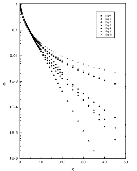
Figure 1: Comparison of $\phi$ from Eqs.(1), (2), (3), (4), (5) and (21).

After inserting the equation (21) into the equations (19) and (18), the lagrangian $L(\phi)$ transforms into an algebraic function $L(\alpha,\beta,\gamma)$ of the variational parameters $\alpha$, $\beta$ and $\gamma$ and the Thomas-Fermi problem turns into minimizing $L(\alpha,\beta,\gamma)$ with respect to these parameters subject to the constraint (17) which is taken into account through a Lagrange multiplier. All calculations, in this work, are performed with the software Maple Release 9.

III RESULTS

The optimum values of the variational parameters $\alpha$, $\beta$ and $\gamma$, obtained by minimizing the lagrangian (18) taking into account the subsidiary condition (17), are respectively equal to 0.7280642371, -0.5430794693 and 0.3612163121. The obtained trial function (Eq.(21)), with these universal parameters, reproduces accurately the numerical solution 11 of the Thomas-Fermi equation (14), in the range $0\leq x\leq 50$, in comparison with the equations (1), (2), (3), (4) and (5) as it is shown in Fig. 1 and Tab. I. The mean error of our calculations, calculated on 67 points in the range $0\leq x\leq 50$ with respect to the numerical solution, is about 2 % , while the other calculations have a mean error greater than 17 %.

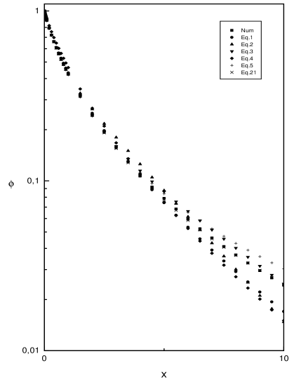
Figure 2: Comparison of $\phi$ from Eqs.(1), (2), (3), (4), (5) and (21) in the main region of the screening potential.

Table 1: Comparison of the values of $\phi$ from numerical solution and equations (1), (2), (3), (4), (5) and (21). R.E(%) is the relative error with respect to the numerical solution

x	Num	Eq.(1)	R.E(%)	Eq.(2)	R.E(%)	Eq.(3)	R.E(%)	Eq.(4)	R.E(%)	Eq.(5)	R.E(%)	Eq.(21)	R.E(%)
0	1	1	0.00	1	0.00	1	0.00	1	0.00	1	0.00	1	0.00
0.001	0.9985	0.9983	-0.02	0.9988	0.03	0.9986	0.01	0.9987	0.02	0.9982	-0.03	0.9984	-0.01
0.002	0.9969	0.9966	-0.03	0.9975	0.06	0.9972	0.03	0.9975	0.06	0.9966	-0.03	0.9969	0.00
0.003	0.9955	0.9949	-0.06	0.9963	0.08	0.9958	0.03	0.9962	0.07	0.9950	-0.05	0.9954	-0.01
0.004	0.994	0.9933	-0.07	0.9951	0.11	0.9944	0.04	0.9950	0.10	0.9935	-0.05	0.9939	-0.01
0.005	0.9925	0.9917	-0.08	0.9939	0.14	0.9930	0.05	0.9938	0.13	0.9920	-0.05	0.9924	-0.01
0.006	0.9911	0.9901	-0.10	0.9926	0.15	0.9917	0.06	0.9926	0.15	0.9906	-0.05	0.9910	-0.01
0.007	0.9897	0.9886	-0.11	0.9914	0.17	0.9903	0.06	0.9914	0.17	0.9891	-0.06	0.9895	-0.02
0.008	0.9882	0.9870	-0.12	0.9902	0.20	0.9889	0.07	0.9902	0.20	0.9877	-0.05	0.9881	-0.01
0.009	0.9868	0.9855	-0.13	0.9890	0.22	0.9876	0.08	0.9890	0.22	0.9863	-0.05	0.9867	-0.01
0.01	0.9854	0.9840	-0.14	0.9878	0.24	0.9862	0.08	0.9878	0.25	0.9849	-0.05	0.9853	-0.01
0.05	0.9352	0.9314	-0.41	0.9412	0.64	0.9357	0.06	0.9451	1.06	0.9359	0.07	0.9348	-0.05
0.09	0.8919	0.8874	-0.51	0.8983	0.72	0.8914	-0.05	0.9076	1.76	0.8933	0.16	0.8913	-0.06
0.4	0.6596	0.6609	0.19	0.6557	-0.59	0.6607	0.16	0.6972	5.71	0.6598	0.03	0.6601	0.08
0.8	0.4849	0.4920	1.47	0.4816	-0.68	0.4867	0.36	0.5268	8.63	0.4821	-0.57	0.4858	0.19
1.5	0.3148	0.3233	2.70	0.3276	4.06	0.3136	-0.38	0.3476	10.43	0.3116	-1.01	0.3147	-0.03
5	0.0788	0.0743	-5.71	0.0877	11.25	0.0861	9.30	0.0749	-4.96	0.0838	6.34	0.0774	-1.73
10	0.0243	0.0170	-30.06	0.0147	-39.33	0.0247	1.73	0.0150	-38.11	0.0304	25.01	0.0247	1.44
15	0.0108	0.0052	-51.53	0.0025	-77.04	0.0074	-31.56	0.0041	-62.31	0.0157	45.66	0.0116	7.78
20	0.00578	0.00190	-67.13	0.00042	-92.78	0.00221	-61.72	0.00130	-77.51	0.00965	66.93	0.00653	12.98
37.5	0.00131	0.00011	-91.70	8.14E-07	-99.94	3.25E-05	-97.52	5.03E-05	-96.16	3.17E-03	141.61	0.00140	6.87
45	8.28E-04	3.88E-05	-95.31	5.62E-08	-99.99	5.32E-06	-99.36	1.54E-05	-98.14	2.27E-03	174.18	7.92E-04	-4.37
50	6.32E-04	2.04E-05	-96.77	9.45E-09	-100	1.59E-06	-99.75	7.36E-06	-98.84	1.87E-03	196.02	5.50E-04	-12.90

In the main region of the screening potential of Thomas-Fermi $(0\leq x\leq 10)$, our function is even more precise than all other proposed functions as one can see from Fig. 2 and Tab. I. The mean error of our calculations, calculated on 47 points in this region, is equal to 0.28 %, while the Eq.(2) has a mean error equal to 1.13 % and the Eqs.(1), (3), (4) and (5) have a mean error greater than 2.5 %.

The derivative of our function (Eq.(21)) at $x=0$ is equal to -1.61623647 which is close to the numerical derivative: -1.58807102 11 . The relative error is less than 2 %, while the equations (1), (2), (3) and (4) give a result with an error greater than 11 % with respect to the numerical derivative and the Eq.(5) has an infinite derivative at x = 0.
To test the efficiency of the different trial functions, given by the equations (1), (2), (3), (4) and (21), we have calculated the total ionization energy of heavy atoms following the relation 12 :

$$E=\left(\frac{12}{7}\right)\left(\frac{2}{9\pi^{2}}\right)^{1/3}\left(\frac{d\phi}{dx}\right)_{x=0}Z^{7/3},$$ (22)

in hartrees $(e^{2}/a_{B})$ and the obtained results, presented in Tab. II, are compared with those of Hartree-Fock (HF) 13 . The Eq.(5) cannot be used because of its infinite derivative at $x=0$. From Tab. II, one can see that our results are fairly better than those obtained from the Eqs.(1), (2), (3) and (4). The precision of our calculations rises with the atomic number Z, on the contrary of the other calculations performed with the Eqs.(1), (2), (3) and (4), so our trial function is more suited for heavy atoms.

IV CONCLUSION

The proposed new trial function (Eq.(21)) provides a more satisfactory approximation for the solution of the Thomas-Fermi equation for neutral atoms than all other previousely proposed analytical solutions. The results obtained for the total ionization energies of heavy atoms agree with the Hartree-Fock data and are more precise than those calculated with the Eqs.(1), (2), (3) and (4). The proposed solution (Eq.(21)) can be used to calculate, with high precision, other atomic characteristics of heavy atoms.

Table 2: Comparison of total ionization energies in units $(e^{2}/a_{B})$ from HF and equations (1), (2), (3), (4) and (21).

Z	HF	Eq.(1)	Errors(%)	Eq.(2)	Errors(%)	Eq.(3)	Errors(%)	Eq.(4)	Errors(%)	Eq.(21)	Errors(%)
92	28070	33562	19.6	22864	-18.5	25972	-7.5	24392	-13.1	29894	6.5
93	28866	34419	19.2	23448	-18.8	26636	-7.7	25015	-13.3	30658	6.2
94	29678	35289	18.9	24040	-19.0	27309	-8.0	25647	-13.6	31433	5.9
95	30506	36171	18.6	24641	-19.2	27992	-8.2	26288	-13.8	32219	5.6
96	31351	37066	18.2	25251	-19.5	28684	-8.5	26938	-14.1	33015	5.3
97	32213	37973	17.9	25869	-19.7	29386	-8.8	27598	-14.3	33823	5.0
98	33093	38893	17.5	26495	-19.9	30098	-9.1	28266	-14.6	34643	4.7
99	33990	39825	17.2	27130	-20.2	30819	-9.3	28944	-14.8	35473	4.4
100	34905	40770	16.8	27774	-20.4	31550	-9.6	29631	-15.1	36315	4.0
101	35839	41727	16.4	28426	-20.7	32292	-9.9	30327	-15.4	37168	3.7
102	36793	42698	16.0	29088	-20.9	33042	-10.2	31032	-15.7	38032	3.4
103	37766	43681	15.7	29757	-21.2	33803	-10.5	31746	-15.9	38908	3.0
104	38758	44677	15.3	30436	-21.5	34574	-10.8	32470	-16.2	39795	2.7
105	39772	45686	14.9	31123	-21.7	35355	-11.1	33203	-16.5	40694	2.3
106	40806	46707	14.5	31819	-22.0	36145	-11.4	33946	-16.8	41604	2.0
107	41862	47742	14.0	32524	-22.3	36946	-11.7	34698	-17.1	42525	1.6
108	42941	48790	13.6	33238	-22.6	37757	-12.1	35459	-17.4	43458	1.2
109	44042	49850	13.2	33960	-22.9	38578	-12.4	36230	-17.7	44403	0.8

References

- (1) E. D. Grezia and S. Esposito, DSF-6/2004, Physics/04606030.
- (2) E. Roberts, Phys. Rev. 170, 8 (1968).
- (3) P. Csavinsky, Phys. Rev.A 8, 1688 (1973).
- (4) R. N. Kesarwani and Y. P. Varshni, Phys. Rev. A 23, 991 (1981).
- (5) O. B. Firsov, Zh. Eksp. Teo. Fiz.32, 696 (1957)[Sov. Phys.-JETP5, 1192 (1957); 6, 534 (1958)].
- (6) M. Wu, Phys. Rev. A 26, 57 (1982).
- (7) M. Desaix, D. Anderson and M. Lisak, Eur. J. Phys. 24 (2004) 699-705.
- (8) N. Anderson, A. M. Arthurs and P. D. Robinson, Nuovo Cimento 57, 523 (1968).
- (9) W. p. Wang and R. G. Parr, Phys. Rev. A 16, 891 (1977).
- (10) E. K. U. Gross and R. M. Dreiler, Phys. Rev. A 20, 1798 (1979).
- (11) Paul S. Lee and Ta-You Wu, Chinese Journal of Physics, Vol.35, N 6-11, 1997.
- (12) P. Gombas, Encyclopedia of Physics, edited by S. Fl gge ( Springer, Berlin, 1956), Vol. XXXVI.
- (13) L. Visschen and K. G. Dyall, Atom. Data. Nucl. Data. Tabl., 67 (1997) 207.