Analysis of on-line learning
when a moving teacher goes around a true teacher

Abstract

In the framework of on-line learning, a learning machine might move around a teacher due to the differences in structures or output functions between the teacher and the learning machine or due to noises. The generalization performance of a new student supervised by a moving machine has been analyzed. A model composed of a true teacher, a moving teacher and a student that are all linear perceptrons with noises has been treated analytically using statistical mechanics. It has been proven that the generalization errors of a student can be smaller than that of a moving teacher, even if the student only uses examples from the moving teacher.

Key-words: on-line learning, generalization error, moving teacher, true teacher, unlearnable case

1 Introduction

Learning is to infer the underlying rules that dominate data generation using observed data. The observed data are input-output pairs from a teacher. They are called examples. Learning can be roughly classified into batch learning and on-line learning [1]. In batch learning, some given examples are used repeatedly. In this paradigm, a student becomes to give correct answers after training if that student has an adequate degree of freedom. However, it is necessary to have a long amount of time and a large memory in which many examples may be stored. On the contrary, examples used once are discarded in on-line learning. In this case, a student cannot give correct answers for all examples used in training. However, there are some merits, for example, a large memory for storing many examples isn’t necessary and it is possible to follow a time variant teacher.

Recently, we [6, 7] have analyzed the generalization performance of ensemble learning [2, 3, 4, 5] in a framework of on-line learning using a statistical mechanical method [1, 8]. In that process, the following points are proven subsidiarily. The generalization error doesn’t approach zero when the student is a simple perceptron and the teacher is a committee machine [11] or a non-monotonic perceptron [12]. Therefore, models like these can be called unlearnable cases [9, 10]. The behavior of a student in an unlearnable case depends on the learning rule. That is, the student vector asymptotically converges in one direction using Hebbian learning. On the contrary, the student vector doesn’t converge in one direction but continues moving using perceptron learning or AdaTron learning. In the case of a non-monotonic teacher, the student’s behavior can be expressed by continuing to go around the teacher, keeping a constant direction cosine with the teacher.

Considering the applications of statistical learning theories, investigating the system behaviors of unlearnable cases is very significant since real world problems seem to include many unlearnable cases. In addition, a learning machine may continue going around a teacher in the unlearnable cases as mentioned above. Here, let us consider a new student that is supervised by a moving learning machine. That is, we consider a student that uses the input-output pairs of a moving teacher as training examples and we investigate the generalization performance of a student with a true teacher. Note that the examples used by the student are only from the moving teacher and the student can’t directly observe the outputs of the true teacher. In a real human society, a teacher that can be observed by a student doesn’t always present the correct answer. In many cases, the teacher is learning and continues to vary. Therefore, the analysis of such a model is interesting for considering the analogies between statistical learning theories and a real society.

In this paper, we treat a model in which a true teacher, a moving teacher and a student are all linear perceptrons [6] with noises, as the simplest model in which a moving teacher continues going around a true teacher. We calculate the order parameters and the generalization errors analytically using a statistical mechanical method in the framework of on-line learning. As a result, it is proven that a student’s generalization errors can be smaller than that of the moving teacher. That means the student can be cleverer than the moving teacher even though the student uses only the examples of the moving teacher.

2 Model

Three linear perceptrons are treated in this paper: a true teacher, a moving teacher and a student. Their connection weights are $\mbox{\boldmath$A$},\mbox{\boldmath$B$}$ and $J$, respectively. For simplicity, the connection weight of the true teacher, that of the moving teacher and that of the student are simply called the true teacher, the moving teacher, and the student, respectively. The true teacher $\mbox{\boldmath$A$}=(A_{1},\ldots,A_{N})$, the moving teacher $\mbox{\boldmath$B$}=(B_{1},\ldots,B_{N})$, the student $\mbox{\boldmath$J$}=(J_{1},\ldots,J_{N})$, and input $\mbox{\boldmath$x$}=(x_{1},\ldots,x_{N})$ are $N$ dimensional vectors. Each component $A_{i}$ of $A$ is drawn from ${\cal N}(0,1)$ independently and fixed, where ${\cal N}(0,1)$ denotes the Gaussian distribution with a mean of zero and a variance unity. Each of the components $B_{i}^{0},J_{i}^{0}$ of the initial values of $\mbox{\boldmath$B$},\mbox{\boldmath$J$}$ are drawn from ${\cal N}(0,1)$ independently. Each component $x_{i}$ of $x$ is drawn from ${\cal N}(0,1/N)$ independently. Thus,

$$\left\langle A_{i}\right\rangle = 0,\ \left\langle(A_{i})^{2}\right\rangle=1,$$ (1)

$$\left\langle B_{i}^{0}\right\rangle = 0,\ \left\langle(B_{i}^{0})^{2}\right\rangle=1,$$ (2)

$$\left\langle J_{i}^{0}\right\rangle = 0,\ \left\langle(J_{i}^{0})^{2}\right\rangle=1,$$ (3)

$$\left\langle x_{i}\right\rangle = 0,\ \left\langle(x_{i})^{2}\right\rangle=\frac{1}{N},$$ (4)

where $\langle\cdot\rangle$ denotes a mean.

In this paper, the thermodynamic limit $N\rightarrow\infty$ is also treated. Therefore,

$$\|\mbox{\boldmath$A$}\|=\sqrt{N},\ \ \|\mbox{\boldmath$B$}^{0}\|=\sqrt{N},\ \ \|\mbox{\boldmath$J$}^{0}\|=\sqrt{N},\ \ \|\mbox{\boldmath$x$}\|=1,$$ (5)

where $\|\cdot\|$ denotes a vector norm. Generally, norms $\|\mbox{\boldmath$B$}\|$ and $\|\mbox{\boldmath$J$}\|$ of the moving teacher and the student change as the time step proceeds. Therefore, the ratios $l_{B}$ and $l_{J}$ of the norms to $\sqrt{N}$ are introduced and are called the length of the moving teacher and the length of the student. That is, $\|\mbox{\boldmath$B$}\|=l_{B}\sqrt{N}$ C $\|\mbox{\boldmath$J$}\|=l_{J}\sqrt{N}$.

The outputs of the true teacher, the moving teacher, and the student are $y^{m}+n_{A}^{m}$, $v^{m}l_{B}^{m}+n_{B}^{m}$, and $u^{m}l_{J}^{m}+n_{J}^{m}$, respectively. Here,

$$y^{m} = \mbox{\boldmath$A$}\cdot\mbox{\boldmath$x$}^{m},$$ (6)

$$v^{m}l_{B}^{m} = \mbox{\boldmath$B$}^{m}\cdot\mbox{\boldmath$x$}^{m},$$ (7)

$$u^{m}l_{J}^{m} = \mbox{\boldmath$J$}^{m}\cdot\mbox{\boldmath$x$}^{m},$$ (8)

and

$$n_{A}^{m} \sim {\cal N}(0,\sigma_{A}^{2}),$$ (9)

$$n_{B}^{m} \sim {\cal N}(0,\sigma_{B}^{2}),$$ (10)

$$n_{J}^{m} \sim {\cal N}(0,\sigma_{J}^{2}).$$ (11)

where $m$ denotes the time step. That is, the outputs of the true teacher, the moving teacher and the student include independent Gaussian noises with variances of $\sigma_{A}^{2},\sigma_{B}^{2}$, and $\sigma_{J}^{2}$, respectively. Then, the $y^{m}$, $v^{m}$, and $u^{m}$ of Eqs.(6)–(8) obey the Gaussian distributions with a mean of zero and a variance unity.

In the model treated in this paper, the moving teacher $B$ is updated using an input $x$ and an output of the true teacher $A$ for the input $x$. The student $J$ is updated by using an input $x$ and an output of the moving teacher $B$ for the input $x$. Let us define an error between the true teacher and the moving teacher by the squared error of their outputs. That is,

$$\epsilon_{B}^{m}\equiv\frac{1}{2}\left(y^{m}+n_{A}^{m}-v^{m}l_{B}^{m}-n_{B}^{m}\right)^{2}.$$ (12)

The moving teacher is considered to use the gradient method for learning. That is,

$$\mbox{\boldmath$B$}^{m+1} = \mbox{\boldmath$B$}^{m}-\eta_{B}\frac{\partial\epsilon_{B}^{m}}{\partial\mbox{\boldmath$B$}^{m}}$$ (13)

$$= \mbox{\boldmath$B$}^{m}+\eta_{B}\left(y^{m}+n_{A}^{m}-v^{m}l_{B}^{m}-n_{B}^{m}\right)\mbox{\boldmath$x$}^{m},$$ (14)

where, $\eta_{B}$ denotes the learning rate of the moving teacher and is a constant number.

In the same manner, let us define an error between the moving teacher and the student by the squared error of their outputs. That is,

$$\epsilon_{BJ}^{m}\equiv\frac{1}{2}\left(v^{m}l_{B}^{m}+n_{B}^{m}-u^{m}l_{J}^{m}-n_{J}^{m}\right)^{2}.$$ (15)

The student is considered to use the gradient method for learning. That is,

$$\mbox{\boldmath$J$}^{m+1} = \mbox{\boldmath$J$}^{m}-\eta_{J}\frac{\partial\epsilon_{BJ}^{m}}{\partial\mbox{\boldmath$J$}^{m}}$$ (16)

$$= \mbox{\boldmath$J$}^{m}+\eta_{J}\left(v^{m}l_{B}^{m}+n_{B}^{m}-u^{m}l_{J}^{m}-n_{J}^{m}\right)\mbox{\boldmath$x$}^{m},$$ (17)

where, $\eta_{J}$ denotes a learning rate of the student and is a constant number.

Generalizing the learning rules, Eqs.(14) and (17) can be expressed as

$$\mbox{\boldmath$B$}^{m+1} = \mbox{\boldmath$B$}^{m}+g\left(y^{m}+n_{A}^{m},v^{m}l_{B}^{m}+n_{B}^{m}\right)\mbox{\boldmath$x$}^{m},$$ (18)

$$\mbox{\boldmath$J$}^{m+1} = \mbox{\boldmath$J$}^{m}+f\left(v^{m}l_{B}^{m}+n_{B}^{m},u^{m}l_{J}^{m}+n_{J}^{m}\right)\mbox{\boldmath$x$}^{m},$$ (19)

respectively.

Let us define an error between the true teacher and the student by the squared error of their outputs. That is,

$$\epsilon_{J}^{m}\equiv\frac{1}{2}\left(y^{m}+n_{A}^{m}-u^{m}l_{J}^{m}-n_{J}^{m}\right)^{2}.$$ (20)

3 Theory

3.1 Generalization Error

One purpose of a statistical learning theory is to theoretically obtain generalization errors. Since a generalization error is the mean of errors for the true teacher over the distribution of the new input and noises, the generalization error $\epsilon_{Bg}$ of the moving teacher and $\epsilon_{Jg}$ of the student are calculated as follows. The superscripts $m$, which represent the time steps, are omitted for simplicity.

$$\epsilon_{Bg} = \int d\mbox{\boldmath$x$}dn_{A}dn_{B}P(\mbox{\boldmath$x$},n_{A},n_{B})\epsilon_{B}$$ (22)

$$= \int dydvdn_{A}dn_{B}P(y,v,n_{A},n_{B})$$

$$\times\frac{1}{2}\left(y+n_{A}-vl_{B}-n_{B}\right)^{2}$$

$$= \frac{1}{2}\left(-2R_{B}l_{B}+(l_{B})^{2}+1+\sigma_{A}^{2}+\sigma_{B}^{2}\right),$$ (23)

$$\epsilon_{Jg} = \int d\mbox{\boldmath$x$}dn_{A}dn_{J}P(\mbox{\boldmath$x$},n_{A},n_{J})\epsilon_{J}$$ (25)

$$= \int dydudn_{A}dn_{J}P(y,u,n_{A},n_{J})$$

$$\times\frac{1}{2}\left(y+n_{A}-ul_{J}-n_{J}\right)^{2}$$

$$= \frac{1}{2}\left(-2R_{J}l_{J}+(l_{J})^{2}+1+\sigma_{A}^{2}+\sigma_{J}^{2}\right).$$ (26)

In addition, let us calculate the mean $\epsilon_{BJg}$ of the error between the student and the moving teacher as follows:

$$\epsilon_{BJg} = \int d\mbox{\boldmath$x$}dn_{B}dn_{J}P(\mbox{\boldmath$x$},n_{B},n_{J})\epsilon_{BJ}$$ (28)

$$= \int dvdudn_{B}dn_{J}P(v,u,n_{B},n_{J})$$

$$\times\frac{1}{2}\left(vl_{B}+n_{B}-ul_{J}-n_{J}\right)^{2}$$

$$= \frac{1}{2}\left(-2R_{BJ}l_{B}l_{J}+(l_{J})^{2}+(l_{B})^{2}+\sigma_{B}^{2}+\sigma_{J}^{2}\right).$$ (29)

Here, the integration has been executed using the following: $y$, $v$ and $u$ obeys ${\cal N}(0,1)$. The covariance between $y$ and $v$ is $R_{B}$, between $y$ and $u$ is $R_{J}$, and between $v$ and $u$ is $R_{BJ}$, where

$$R_{B} \equiv \frac{\mbox{\boldmath$A$}\cdot\mbox{\boldmath$B$}}{\|\mbox{\boldmath$A$}\|\|\mbox{\boldmath$B$}\|},\ \ \ R_{J}\equiv\frac{\mbox{\boldmath$A$}\cdot\mbox{\boldmath$J$}}{\|\mbox{\boldmath$A$}\|\|\mbox{\boldmath$J$}\|},\ \ \ R_{BJ}\equiv\frac{\mbox{\boldmath$B$}\cdot\mbox{\boldmath$J$}}{\|\mbox{\boldmath$B$}\|\|\mbox{\boldmath$J$}\|}.$$ (30)

Eq.(30) means that $R_{B}$, $R_{J}$, and $R_{BJ}$ are direction cosines. $n_{A}$, $n_{B}$, and $n_{J}$ are all independent with other probabilistic variables. The true teacher $A$, the moving teacher $B$, the student $J$, and the relationship among $R_{B},R_{J}$, and $R_{BJ}$ are shown in Fig.1.

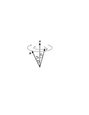
Figure 1: True teacher $A$, moving teacher $B$ and student $J$. $R_{B},R_{J}$, and $R_{BJ}$ are direction cosines.

3.2 Differential equations of order parameters and their analytical solutions

To make analysis easy, the following auxiliary order parameters are introduced:

$$r_{B} \equiv R_{B}l_{B},$$ (31)

$$r_{J} \equiv R_{J}l_{J},$$ (32)

$$r_{BJ} \equiv R_{BJ}l_{B}l_{J}.$$ (33)

Simultaneous differential equations in deterministic forms [8] have been obtained that describe the dynamical behaviors of order parameters based on self-averaging in the thermodynamic limits as follows:

$$\frac{dr_{B}}{dt} = \langle gy\rangle,$$ (34)

$$\frac{dr_{J}}{dt} = \langle fy\rangle,$$ (35)

$$\frac{dr_{BJ}}{dt} = l_{J}\langle gu\rangle+l_{B}\langle fv\rangle+\langle gf\rangle,$$ (36)

$$\frac{dl_{B}}{dt} = \langle gv\rangle+\frac{\langle g^{2}\rangle}{2l_{B}},$$ (37)

$$\frac{dl_{J}}{dt} = \langle fu\rangle+\frac{\langle f^{2}\rangle}{2l_{J}}.$$ (38)

Since linear perceptrons are treated in this paper, the sample averages that appeared in the above equations can be calculated easily as follows:

$$\langle gu\rangle = \eta_{B}(r_{J}-r_{BJ})/l_{J},$$ (39)

$$\langle fv\rangle = \eta_{J}(l_{B}-r_{BJ}/l_{B}),$$ (40)

$$\langle gf\rangle = \eta_{B}\eta_{J}(r_{B}-r_{J}-l_{B}^{2}+r_{BJ}-\sigma_{B}^{2}),$$ (41)

$$\langle fy\rangle = \eta_{J}(r_{B}-r_{J}),$$ (42)

$$\langle gy\rangle = \eta_{B}(1-r_{B}),$$ (43)

$$\langle gv\rangle = \eta_{B}(r_{B}/l_{B}-l_{B}),$$ (44)

$$\langle g^{2}\rangle = \eta_{B}^{2}(1+\sigma_{A}^{2}+\sigma_{B}^{2}+l_{B}^{2}-2r_{B}),$$ (45)

$$\langle fu\rangle = \eta_{J}(r_{BJ}/l_{J}-l_{J}),$$ (46)

$$\langle f^{2}\rangle = \eta_{J}^{2}(l_{B}^{2}+l_{J}^{2}+\sigma_{B}^{2}+\sigma_{J}^{2}-2r_{BJ}).$$ (47)

Since each components of the true teacher $A$, the initial value of the moving teacher $B$, and the initial value of the student $J$ are drawn from ${\cal N}(0,1)$ independently and because the thermodynamic limit $N\rightarrow\infty$ is also treated, they are all orthogonal to each other in the initial state. That is,

$$R_{B}^{0}=R_{J}^{0}=R_{BJ}^{0}=0.$$ (48)

In addition,

$$l_{B}^{0}=l_{J}^{0}=1.$$ (49)

By using Eqs.(39)–(49), the simultaneous differential equations Eqs.(34)–(38) can be solved analytically as follows:

$$r_{B} = 1-e^{-\eta_{B}t},$$ (50)

$$r_{J} = 1+\frac{\eta_{B}}{\eta_{J}-\eta_{B}}e^{-\eta_{J}t}-\frac{\eta_{J}}{\eta_{J}-\eta_{B}}e^{-\eta_{B}t},$$ (51)

$$r_{BJ} = -\frac{D}{\eta_{B}\eta_{J}-\eta_{B}-\eta_{J}}$$ (52)

$$+ \frac{2\eta_{J}-\eta_{B}}{\eta_{B}-\eta_{J}}e^{-\eta_{B}t}+\frac{\eta_{B}}{\eta_{J}-\eta_{B}}e^{-\eta_{J}t}$$

$$+ \frac{\eta_{J}}{\eta_{J}-\eta_{B}}Ce^{\eta_{B}(\eta_{B}-2)t}+Ee^{(\eta_{B}\eta_{J}-\eta_{B}-\eta_{J})t},$$

$$l_{B}^{2} = 3-C-2e^{-\eta_{B}t}+Ce^{\eta_{B}(\eta_{B}-2)t},$$ (53)

$$l_{J}^{2} = -\frac{G}{\eta_{J}(\eta_{J}-2)}$$ (54)

$$+ \frac{F}{\eta_{B}(\eta_{B}-2)-\eta_{J}(\eta_{J}-2)}e^{\eta_{B}(\eta_{B}-2)t}$$

$$+ \frac{2\eta_{B}}{\eta_{J}-\eta_{B}}e^{-\eta_{J}t}-\frac{2\eta_{J}}{\eta_{J}-\eta_{B}}e^{-\eta_{B}t}$$

$$- \frac{2\eta_{J}E}{\eta_{B}-\eta_{J}}e^{(\eta_{B}\eta_{J}-\eta_{B}-\eta_{J})t}+He^{\eta_{J}(\eta_{J}-2)t},$$

where

$$C = 2-\frac{\eta_{B}}{2-\eta_{B}}(\sigma_{A}^{2}+\sigma_{B}^{2}),$$ (55)

$$D = \eta_{B}(1-\eta_{J}\sigma_{B}^{2})+\eta_{J}(1-\eta_{B})\left(3-C\right),$$ (56)

$$E = \frac{-\eta_{B}^{2}\eta_{J}}{(\eta_{J}-\eta_{B})(\eta_{B}\eta_{J}-\eta_{B}-\eta_{J})}(\sigma_{A}^{2}+\sigma_{B}^{2})$$ (57)

$$- \frac{2\eta_{B}}{\eta_{J}-\eta_{B}}+\frac{\eta_{B}(1-\eta_{J}\sigma_{B}^{2})}{\eta_{B}\eta_{J}-\eta_{B}-\eta_{J}},$$

$$F = \eta_{J}^{2}\frac{\eta_{B}+\eta_{J}-2}{\eta_{B}-\eta_{J}}C,$$ (58)

$$G = \eta_{J}^{2}\left(3+\sigma_{B}^{2}+\sigma_{J}^{2}-C\right)-\frac{2\eta_{J}(1-\eta_{J})D}{\eta_{B}\eta_{J}-\eta_{B}-\eta_{J}},$$ (59)

$$H = 3-\frac{F}{\eta_{B}(\eta_{B}-2)-\eta_{J}(\eta_{J}-2)}$$ (60)

$$+ \frac{G}{\eta_{J}(\eta_{J}-2)}+\frac{2\eta_{J}}{\eta_{B}-\eta_{J}}E.$$

4 Results and discussion

The dynamical behaviors of the generalization errors $\epsilon_{Bg},\epsilon_{Jg}$ and $\epsilon_{BJg}$ have been obtained analytically by solving Eqs.(23), (26), (29), (31)–(33) , and (50)–(60). Figures 2 and 3 show the analytical results and the corresponding simulation results, where $N=10^{3}$. In the computer simulations, $\epsilon_{Bg},\epsilon_{Jg}$, and $\epsilon_{BJg}$ have been obtained by averaging the squared errors for $10^{4}$ random inputs at each time step. The dynamical behaviors of $R$ and $l$ are shown in Figs.4 and 5. In these figures, the curves represent the theoretical results. The dots represent the simulation results. Conditions other than $\eta_{J}$ are common: $\eta_{B}=1.0,\sigma_{A}^{2}=0.2,\sigma_{B}^{2}=0.3$, and $\sigma_{J}^{2}=0.4$. Figures 2 and 4 show the results in the case of $\eta_{J}=1.2$. Figures 3 and 5 show the results in the case of $\eta_{J}=0.3$.

Figure 2: Generalization errors $\epsilon_{Jg}$, $\epsilon_{Bg}$, and $\epsilon_{BJg}$ in the case of $\eta_{J}=1.2$. Theory and computer simulation. Conditions other than $\eta_{J}$ are $\eta_{B}=1.0,\sigma_{A}^{2}=0.2,\sigma_{B}^{2}=0.3$, and $\sigma_{J}^{2}=0.4$.

Figure 3: Generalization errors $\epsilon_{Jg}$, $\epsilon_{Bg}$, and $\epsilon_{BJg}$ in the case of $\eta_{J}=0.3$. Theory and computer simulation. Conditions other than $\eta_{J}$ are $\eta_{B}=1.0,\sigma_{A}^{2}=0.2,\sigma_{B}^{2}=0.3$, and $\sigma_{J}^{2}=0.4$.

Figure 2 shows that the generalization error $\epsilon_{Jg}$ of the student is always larger than the generalization error $\epsilon_{Bg}$ of the moving teacher when the learning rate of student is relatively large, such as $\eta_{J}=1.2$. In addition, the mean $\epsilon_{BJg}$ of the error between the moving teacher and the student is still larger than $\epsilon_{Jg}$. Figure 4 shows that the direction cosine $R_{J}$ between the true teacher and the student is always smaller than the direction cosine $R_{B}$ between the true teacher and the moving teacher.

Figure 4: $R$ and $l$ in the case of $\eta_{J}=1.2$. Theory and computer simulation. Conditions other than $\eta_{J}$ are $\eta_{B}=1.0,\sigma_{A}^{2}=0.2,\sigma_{B}^{2}=0.3$, and $\sigma_{J}^{2}=0.4$.

Figure 5: $R$ and $l$ in the case of $\eta_{J}=0.3$. Theory and computer simulation. Conditions other than $\eta_{J}$ are $\eta_{B}=1.0,\sigma_{A}^{2}=0.2,\sigma_{B}^{2}=0.3$, and $\sigma_{J}^{2}=0.4$.

On the contrary, Fig.3 shows that when the learning rate of the student is relatively small, that is $\eta_{J}=0.3$. Although the generalization error $\epsilon_{Jg}$ of the student is larger than the generalization error $\epsilon_{Bg}$ of the moving teacher in the initial stage of learning, as in the case of $\eta_{J}=1.2$, the size relationship is reversed at $t=4.4$, and after that $\epsilon_{Jg}$ is smaller than $\epsilon_{Bg}$. This means the performance of the student becomes higher than that of the moving teacher. In regard to the direction cosine, Fig.5 shows that though the direction cosine $R_{J}$ between the true teacher and the student is smaller than the direction cosine $R_{B}$ between the true teacher and the moving teacher in the initial stage of learning, the size relationship is reversed at $t=5.2$, and after that, $R_{J}$ grows larger than $R_{B}$. This means that the student gets closer to the true teacher than the moving teacher in spite of the student only observing the moving teacher. The reason why the size relationship reverses at different times in Fig.3 and Fig.5 is that the generalization error depends on not only the direction cosines $R_{B},R_{J}$, and $R_{BJ}$ but also the lengths $l_{B}$ and $l_{J}$ as shown in Figs.(23), (26), and (29) since linear perceptrons are treated and the squared error is adopted as an error in this paper. In any case, these results show that the student can have higher level of performance than the moving teacher. It depends on the learning rate $\eta_{J}$ of the student. This is a very interesting fact.

In addition, both Figs. 4 and 5 show that the direction cosine $R_{BJ}$ between the moving teacher and the student takes a negative value in the initial stage of learning. That is, the angle between the moving teacher and the student once becomes larger than in the initial condition. This means that the student is once delayed. This is also an interesting phenomenon.

Figures 2 – 5 show that $\epsilon_{Bg},\epsilon_{Jg}$, $\epsilon_{BJg}$, $R$, and $l$ almost seem to reach a steady state by $t=20$. The macroscopic behaviors of $t\rightarrow\infty$ can be understood theoretically since the order parameters have been obtained analytically. Focusing on the signs of the powers of the exponential functions in Eqs.(50)–(54), we can see that $\epsilon_{Bg}$ and $\epsilon_{BJg}$ diverge if $0>\eta_{B}$ or $\eta_{B}>2$, and $\epsilon_{BJg}$ and $\epsilon_{Jg}$ diverge if $0>\eta_{J}$ or $\eta_{J}>2$. The steady state values of $\epsilon_{Bg},\epsilon_{Jg}$, $\epsilon_{BJg}$, $R$, and $l$ in the case of $0<\eta_{B},\eta_{J}<2$ can be easily obtained by substituting $t\rightarrow\infty$ in Eqs.(50)–(54). The relationships that are obtained by this operation, between the learning rate $\eta_{J}$ of the student and $\epsilon_{Bg},\epsilon_{Jg}$, $\epsilon_{BJg}$, $R$, and $l$, are shown in Figs. 6, 7, and 8. The conditions other than $\eta_{J}$ are $\eta_{B}=1.0,\sigma_{A}^{2}=0.2,\sigma_{B}^{2}=0.3$, and $\sigma_{J}^{2}=0.4$ that are the same as Figs. 2– 5. The values on $t=50$ are plotted for the simulations. The values are considered to have already reached a steady state.

Figure 6: Steady value of generalization errors $\epsilon_{Bg},\epsilon_{Jg}$ and $\epsilon_{BJg}$. Theory and computer simulation. Conditions other than $\eta_{J}$ are $\eta_{B}=1.0,\sigma_{A}^{2}=0.2,\sigma_{B}^{2}=0.3$, and $\sigma_{J}^{2}=0.4$.

Figure 7: Steady value of $R$. Theory and computer simulation. Conditions other than $\eta_{J}$ are $\eta_{B}=1.0,\sigma_{A}^{2}=0.2,\sigma_{B}^{2}=0.3$, and $\sigma_{J}^{2}=0.4$.

Figure 8: Steady value of $l$. Theory and computer simulation. Conditions other than $\eta_{J}$ are $\eta_{B}=1.0,\sigma_{A}^{2}=0.2,\sigma_{B}^{2}=0.3$, and $\sigma_{J}^{2}=0.4$.

These figures show the following: though the steady generalization error of the student is larger than that of the moving teacher if $\eta_{J}$ is larger than 0.58, the size relationship is reversed if $\eta_{J}$ is smaller than 0.58. This means the student has higher level of performance than the moving teacher when $\eta_{J}$ is smaller than 0.58. In regard to the steady $R$ and the steady $l$, the size relationships are reversed when $\eta_{J}=0.70$. In the limit of $\eta_{J}\rightarrow 0$, $l_{J}$ approaches unity, $R_{BJ}$ approaches $R_{B}$, and $R_{J}$ approaches unity. That is, the student $J$ coincides with the true teacher $A$ in both direction and length when $\eta_{J}\rightarrow 0$. Note that the reason why the generalization error $\epsilon_{Jg}$ of the student isn’t zero in Fig. 6 is that independent noises are added to the true teacher and the student. The phase transition in which $R_{J}$ and $R_{BJ}$ become zero and $l_{J}$, $\epsilon_{BJg}$, and $\epsilon_{Jg}$ diverge on $\eta_{J}=2$ is shown in Figs. 6–8.

5 Conclusion

The generalization errors of a model composed of a true teacher, a moving teacher, and a student that are all linear perceptrons with noises have been obtained analytically using statistical mechanics. It has been proven that the generalization errors of a student can be smaller than that of a moving teacher, even if the student only uses examples from the moving teacher.

References

• [1] Saad, D. (ed.), On-line Learning in Neural Networks, Cambridge University Press, (1998)
• [2] Freund, Y. and Schapire, R.E., “A short introduction to boosting,” Journal of Japanese Society for Artificial Intelligence, 14(5), 771–780 (1999) (in Japanese, translation by Abe, N.)
• [3] http://www.boosting.org/
• [4] Krogh, A. and Sollich, P., “Statistical mechanics of ensemble learning,” Phys. Rev. E, 55(1), 811–825 (1997).
• [5] Urbanczik, R., “Online learning with ensembles,” Phys. Rev. E, 62(1), 1448–1451 (2000).
• [6] Hara, K. and Okada, M., “Ensemble learning of linear perceptron; Online learning theory”, cond-mat/0402069.
• [7] Miyoshi, S., Hara, K. and Okada, M., “Analysis of ensemble learning using simple perceptrons based on online learning theory”, Phys. Rev. E, 71, 036116. March 2005.
• [8] Nishimori, H., “Statistical Physics of Spin Glasses and Information Processing: An Introduction,” Oxford University Press, (2001)
• [9] Inoue, J. and Nishimori, H., “On-line AdaTron learning of a unlearnable rules,” Phys. Rev. E, 55(4), 4544–4551 (1997).
• [10] Inoue, J., Nishimori, H. and Kabashima, Y., “A simple perceptron that learns non-monotonic rules,” cond-mat/9708096 (1997).
• [11] Miyoshi, S., Hara, K. and Okada, M., “Analysis of ensemble learning for committee machine teacher”, Proc. The Seventh Workshop on Information-Based Induction Sciences, pp.178–185, (2004) (in Japanese).
• [12] Miyoshi, S., Hara, K. and Okada, M., “Analysis of ensemble learning for non-monotonic teacher”, IEICE Technical Report, NC2004-214, pp.123–128, (2005) (in Japanese).