Preprint of:
D. K. Gramotnev, T. A. Nieminen and T. A. Hopper
“Extremely asymmetrical scattering in gratings with varying mean structural parameters”
Journal of Modern Optics 49(9), 1567–1585 (2002)

1 Introduction

Previously, it has been demonstrated that scattering in slanted, strip-like, wide (compared to the wavelength) periodic gratings with the scattered wave propagating parallel or almost parallel to the front grating boundary is characterized by a strong resonant increase in the scattered wave amplitude [1–12]. This type of scattering was called extremely asymmetrical scattering (EAS). It has been shown to be radically different from the conventional Bragg scattering in transmitting or reflecting gratings [1–12]. For example, in addition to the strong resonant increase of the scattered wave amplitude at the Bragg frequency, scattering in the geometry of EAS may also be characterized by additional unique strong resonances, such as an additional exceptionally strong resonance in the sidelobe structure at a frequency that is noticeably higher than the Bragg frequency [11], additional unique resonance with respect to angle of scattering if the scattered wave propagates almost parallel to the grating boundaries [12], combinations of strong simultaneous resonances in non-uniform gratings [7–9], etc.

It has also been shown that the diffractional divergence of the scattered wave inside and outside the grating (similar to the divergence of a laser beam of finite aperture) is responsible for all these unique wave effects in the geometry of EAS [2–9,11,12]. The necessity of taking the divergence into account can be seen from the fact that if the divergence is neglected and the scattered wave propagates parallel to a strip-like grating (the geometry of EAS), then this wave must be located within this grating. Thus we would have a scattered beam with aperture equal to the grating width even if the incident wave is a plane wave. This scattered beam must spread outside the grating owing to diffractional divergence. For a more detailed analysis of the role of diffractional divergence in EAS see [2–9,11,12]. Note that when the scattered wave propagates at a significant (usually several degrees) angle with respect to the grating boundaries, the diffractional divergence of the scattered wave can be neglected [12], and we have conventional scattering in transmitting or reflecting gratings.

On the basis of understanding the role of the diffractional divergence for scattering in the EAS geometry, a new powerful method of simple analytical (approximate) analysis of this type of scattering has been introduced and justified [2–9,11,12]. The main advantage of this method is that it is directly applicable to the analysis of all types of waves in different periodic gratings, including surface and guided waves in periodic groove arrays [2–9,11,12]. Even in a complex five-layer structure with non-collinear grating-assisted coupling, the new method allowed accurate analytical analysis of extremely asymmetrical coupling of two optical modes guided by neighbouring optical slabs with a corrugated interface [2]. The analysis of the applicability conditions for the new method, based on physical speculations [12] and rigorous analysis of EAS [10], has demonstrated that this method normally gives excellent agreement with the rigorous theory for gratings with small amplitude. It is these gratings with small amplitude that are of most interest from the viewpoint of EAS since they result in strong resonant increase of the scattered wave amplitude [2–9]. In addition, the new method provides excellent insight into the physical reasons for EAS, which will allow thoughtful selection of optimal structural parameters for future EAS-based devices and techniques.

If required (for example, for very narrow gratings or large grating amplitude), rigorous analysis of EAS of bulk electromagnetic waves can also be carried out by means of one of the known numerically stable rigorous approaches, such as an enhanced T-matrix approach [13,14], S-matrix and R-matrix approaches [15,16], an S-matrix approach using an oblique Cartesian system of coordinates [17], a C method [18] (for EAS of guided modes in corrugation gratings), etc. For example, in a recent paper [10], the enhanced T-matrix approach was used for the rigorous analysis of EAS of bulk TE electromagnetic waves in uniform holographic gratings with constant mean dielectric permittivity. Note, however, that all these rigorous numerical methods do not reveal the main physical reason for the unique pattern of scattering in EAS—the diffractional divergence of the scattered wave.

Since the divergence plays a crucial role for EAS, variations in this divergence are expected to result in substantial variations in the whole pattern of scattering. It is well known that stepwise or gradual variations of mean structural parameters across a laser beam (for example, in nonlinear wave propagation [19]) may result in substantial variations in the diffractional divergence. Therefore, it can be expected that EAS will be unusually sensitive to even small variations of mean structural parameters across the grating.

On the one hand, this unusual sensitivity may present a problem for experimental observations of EAS, since variations of mean structural parameters naturally occur during manufacturing of periodic gratings. For example, etching or ruling processes that are used for the fabrication of strip-like relief gratings on a surface of a planar waveguide usually result in a small reduction of the mean thickness of the waveguide (slab) in the region of the grating. Thus, mean thickness of the guiding slab will experience a step-like variation at the front and rear grating boundaries. Fabrication of holographic gratings for bulk and guided optical waves also results in varying mean dielectric permittivity in the grating. For example, if coherent UV radiation is used for writing a grating in a photosensitive material, the mean dielectric permittivity in the region of the grating will be slightly increased compared with the regions outside the grating that are not affected by the UV radiation. Such small variations of mean structural parameters can normally be ignored in the case of conventional Bragg scattering in transmission and reflection gratings. However, in the case of EAS, these variations may result in very significant changes in the pattern of scattering.

On the other hand, the unusual sensitivity of EAS to small variations of mean structural parameters may be very useful, e.g. for the development of new optical and acoustic sensors and precise measurement techniques. For example, consider EAS of an optical slab mode into another guided mode of the same slab in a strip-like grating on one of the slab interfaces. Deposition of thin films or layers of some substance onto the regions of the slab outside or inside the grating will result in varying mean effective permittivity of the slab at the grating boundaries. Thus, EAS can be used for the detection of such deposited layers (thin film sensors).

However, no theoretical analysis of EAS of optical waves in non-uniform gratings with varying mean structural parameters has been carried out so far.

Therefore, the aim of this paper is to present theoretical (approximate) and numerical (rigorous) analyses of EAS of optical bulk and guided waves in gratings with step-like variations of mean dielectric permittivity (for bulk TE waves) and mean slab thickness (for optical guided TE and TM modes) at the front and rear grating boundaries. The theoretical analysis will be based on the recently developed approximate method allowing for the diffractional divergence of the scattered wave [2–9,12]. It will be used for the investigation of EAS of bulk and guided optical waves in holographic and surface relief gratings, respectively. The rigorous numerical analysis will be presented for bulk TE electromagnetic waves and will be based on the enhanced T-matrix approach developed by Moharam et al. [13,14]. Comparison between the approximate and rigorous results will be carried out. In particular, the unusually strong sensitivity of EAS to small variations in the mean structural parameters at the front and rear grating boundaries will be confirmed and analysed.

2 Structure and methods of analysis

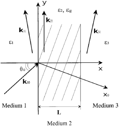
Figure 1: The geometry of EAS in a slanted holographic grating of width $L$ with stepwise variations of the mean permittivity at the front and rear boundaries. The vectors $\mathbf{k}_{11}$, $\mathbf{k}_{21}$, and $\mathbf{k}_{31}$ are the wave vectors of the scattered wave (the first diffracted order) in front, inside, and behind the grating. For EAS of slab modes in a corrugation grating, the plane of the figure is the plane of the slab, and $\epsilon_{1}$, $\epsilon_{2}$, $\epsilon_{3}$, and $\epsilon_{g}$ must be replaced by the slab thicknesses $h_{1}$, $h_{2}$, the mean slab thickness in the grating region $h_{3}$, and the corrugation amplitude $\xi_{g}$, respectively.

The structure analysed in this paper is presented in figure 1. First consider bulk electromagnetic waves in a holographic grating with sinusoidal variations of the dielectric permittivity within a slab of thickness $L$:

$$\epsilon_{s}=\left\{\begin{array}[]{l}\epsilon_{1},\\ \epsilon_{2}+\epsilon_{g}\exp(\mathrm{i}q_{x}x+\mathrm{i}q_{y}y)+\epsilon_{g}^{\ast}\exp(-\mathrm{i}q_{x}x-\mathrm{i}q_{y}y)\\ \epsilon_{3},\end{array},\textrm{for}\right\{\begin{array}[]{l}x<0,\\ 0<x<L,\\ x>L,\end{array}$$ (1)

where the coordinate system is shown in figure 1, $\epsilon_{2}$ is the mean dielectric permittivity in the grating, $\epsilon_{1}$ and $\epsilon_{3}$ are the dielectric permittivities of media 1 and 3 surrounding the grating (figure 1), $\epsilon_{g}$ is the complex amplitude and $\mathbf{q}=(q_{x},q_{y})$ is the reciprocal lattice vector of the grating that is parallel to the $x_{0}$-axis, $q=2\pi/\Lambda$, $\Lambda$ is the period and $L$ is the grating width. The grating is assumed to be infinite along the $y$- and $z$-axes. It is also assumed that dissipation is absent, i.e. $\epsilon_{1,2,3}$ are real and positive (the effect of dissipation on EAS is considered in [20]). The variations of the mean permittivity at the front and rear boundaries are given by$\Delta\epsilon_{1}=\epsilon_{1}-\epsilon_{2}$ and $\Delta\epsilon_{3}=\epsilon_{3}-\epsilon_{2}$ (these values can obviously be real positive or negative). A TE electromagnetic wave with the amplitude of the electric field $S_{10}$ and wave vector $\mathbf{k}_{10}$ is incident onto the grating at an angle $\theta_{10}$ in the $xy$ plane—figure 1 (non-conical scattering).

The solution to the wave equation in the grating can be written in the form of the expansion [13,14,21]:

$$E_{2}(x,y,t)=\sum_{n=-\infty}^{+\infty}E_{2n}(x,y,t),$$ (2)

where

$$E_{2n}(x,y,t)=S_{2n}\exp(\mathrm{i}xk_{2nx}+\mathrm{i}yk_{2ny}-\mathrm{i}\omega t)$$

is the field in each of the inhomogeneous waves in the sum (2) with the $x$-dependent amplitude $S_{2n}(x)$, and $k_{2nx}$ and $k_{2ny}$ are the components of the wave vectors

$$\mathbf{k}_{2n}=\mathbf{k}_{20}-n\mathbf{q},\,\,\,\,(n=0,\pm 1,\pm 2,...).$$ (3)

If for some value of $n$ the magnitude of the wave vector $\mathbf{k}_{2n}$ is equal to $\omega\epsilon^{1/2}_{2}/c$, where $\omega$ is the frequency of the wave, and $c$ is the light speed in vacuum, then the Bragg condition is satisfied for this value of $n$, and the $n$th wave in expansion (2) may have amplitude that is comparable with or even larger than the amplitude of the incident wave (zeroth term in equation (2)).

In this paper it is assumed that the Bragg condition is satisfied precisely for the first diffracted order, i.e. for $n=1$:

$$\mathbf{k}_{21}=\mathbf{k}_{20}-\mathbf{q},$$

where $k_{21}=|\mathbf{k}_{21}|=\omega\epsilon^{1/2}_{2}/c$. The wave vector of the scattered wave (the first diffracted order) in the grating, $\mathbf{k}_{21}$, is parallel to the grating boundaries, i.e. parallel to the $y$-axis (figure 1)—the geometry of EAS [1–10].

In the approximate method of analysis of EAS [2–9,11,12], only the zeroth order (incident wave) and the first order (scattered wave) in equation (2) are considered to be significantly non-zero (the two-wave approximation). It has been shown that the allowance for the second-order $x$-derivative of the scattered wave amplitude in the grating is essential for the correct description of scattering in the geometry of EAS [2–9,11,12]. In the approximate method [2–9,11,12], this second-order derivative is introduced into the coupled wave equations through consideration of the diffractional divergence of the scattered wave, which is one of the main physical reasons for resonant wave effects in the EAS geometry [2–12]. This approach is especially useful for the analysis of EAS of surface and guided waves [2–9, 12], where other methods fail to provide any reasonably simple solutions.

The approximate method developed in [2–9,12] is also directly applicable to the case of non-uniform gratings with step-like variations of the mean structural parameters at the grating boundaries. For example the coupled wave equations in the grating in the geometry of EAS can be written as [4,6,9,12]:

$$\mathrm{d}^{2}S_{21}(x)/\mathrm{d}x^{2}+K_{0}S_{20}(x) = 0,$$

$$\mathrm{d}S_{20}(x)/\mathrm{d}x-\mathrm{i}K_{1}S_{21}(x) = 0,$$ (4)

where

$$K_{0}=-2k_{21}\Gamma_{0}\sin(\eta-\theta_{20}),\,\,\,\,K_{1}=\Gamma_{1}\cos(\eta)/\cos)\theta_{20}),$$ (5)

$\theta_{20}$ is the angle of refraction of the incident wave at the front boundary, $\eta$ is the angle measured from the $x_{0}$-axis to the wave vector of the incident wave $\mathbf{k}_{20}$ in the grating counter-clockwise (figure 1), $\Gamma_{0}$ and $\Gamma_{1}$ are the coupling coefficients that are determined in the conventional coupled wave theories for non-slanted gratings with fringes parallel to the grating boundaries.

The incident wave is partly reflected from the front grating boundary, because the mean dielectric permittivity experiences a step-like variation at $x=0$. However, in the considered approximation, this process of reflection (and refraction) is independent of scattering inside the grating. Therefore, the reflected and refracted waves at the front boundary $x=0$ can be found separately from scattering by means of the well-known Fresnel’s equations for an interface. The determined amplitude $S_{200}$ of the refracted wave at the grating boundary $x=0$, and the angle of refraction $\theta_{20}$ must then be used in equations (4) and (5) as the amplitude and the angle of incidence of the incident wave at this boundary. The wave vector of the incident wave in the grating should be taken as $\mathbf{k}_{20}$—the wave vector of the refracted wave.

Similarly, the reflection of the incident wave at the rear boundary can also be considered separately from the process of scattering. In this case, the incident wave in the grating at $x=L$ is regarded as the wave transmitted through the grating. Then the reflection from the rear boundary will be the reflection of the transmitted wave from this boundary, which (in the approximate method of analysis [2–9,12]) has no effect on the process of scattering.

It can also be seen that if $\epsilon_{2}\neq\epsilon_{1},\epsilon_{3}$, then the scattered wave outside the grating should not necessarily propagate parallel to the grating boundaries, even if this is the case inside the grating (figure 1). In general, the solutions for the scattered wave outside the grating are

$$E_{11}(x,y,t) = A_{0}\exp(\mathrm{i}k_{11y}y-\mathrm{i}k{11x}x-\mathrm{i}\omega t),$$

$$E_{31}(x,y,t) = B_{0}\exp(\mathrm{i}k_{31y}y+\mathrm{i}k_{31x}x-\mathrm{i}\omega t),$$ (6)

where $A_{0}$ and $B_{0}$ are the amplitudes of the scattered waves in media 1 and 3, respectively, $k_{11y}=k_{31y}=k_{21}$,

$$k_{11x}=(k^{2}_{11}-k^{2}_{21})^{1/2},\,\,\,\,k_{31x}=(k^{2}_{31}-k^{2}_{21})^{1/2},$$ (7)

where $k_{11}=\omega\epsilon^{1/2}_{1}/c$, $k_{31}=\omega\epsilon^{1/2}_{3}/c$, and $k_{11x}$ and $k_{31x}$ are chosen positive real or positive imaginary. Note that in the rigorous analysis, equations (6) are replaced by the Rayleigh expansions of the electric field in the regions $x<0$ and $x>L$ [13–16,18,21]. In this case the waves with amplitudes $A_{0}$ and $B_{0}$ (equations (6)) are the first diffracted orders in these expansions.

In the two-wave approximation, the boundary conditions at the grating boundaries can then be written as [2–9,12]:

$$S_{20}|_{x=0}=S_{200},S_{21}|_{x=0}=A_{0},(\mathrm{d}E_{21}/\mathrm{d}x)_{x=0}=(\mathrm{d}E_{11}/\mathrm{d}x)_{x=0},$$

$$E_{21}|_{x=L}=E_{31}|_{x=L},(\mathrm{d}E_{21}/\mathrm{d}x)_{x=L}=(\mathrm{d}E_{31}/\mathrm{d}x)_{x=L}.$$ (8)

Note again that the refraction of the incident (transmitted) waves at the front and rear boundaries of the grating has not been considered when writing boundary conditions (8).

For the rigorous theory, the boundary conditions at the grating boundaries are given in [13,14,21].

Boundary conditions (8) determine unknown wave amplitudes $A_{0}$, $B_{0}$, and three constants of integration in the solutions to the coupled wave equations (4) in the grating region [2–6]. These constants determine the incident and scattered wave amplitudes inside and outside the grating (for the explicit form of the solutions see [2–6]).

3 Numerical results

The numerical results of the approximate and rigorous analyses of EAS in gratings described by equation (1) are presented in this section for bulk TE electromagnetic waves. As has been indicated in [6–9,11,12], there are two typical patterns of EAS, which correspond to narrow and wide gratings. Narrow gratings are those whose widths are less than a critical width $L_{c}$, wide gratings are those with widths larger than $L_{c}$ [6–9,11,12]. Physically, $L_{c}/2$ is the distance within which the scattered wave (beam) can be spread across the grating (i.e. in the direction normal to the wave propagation) by means of the diffractional divergence, before being re-scattered by the grating [7–9]. Simple methods of determination of the critical width were developed in [7, 9]. This critical width is extremely important for scattering in the geometry of EAS. It appears to determine numerous resonant effects in uniform and non-uniform gratings [7– 9,11,12]. Strong differences in the patterns of scattering will also be demonstrated here for EAS in narrow and wide gratings with step-like variations of the mean structural parameters.

3.1 Narrow gratings

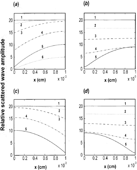
Figure 2: The $x$-dependencies of relative amplitudes $|S_{21}(x)/S_{10}|$ of the scattered bulk TE electromagnetic wave in the holographic grating with the parameters: $\epsilon_{2}=5$, $\epsilon_{g}=5\times 10^{-3}$, $L=10\mu$, $\theta_{10}=\pi/4$, $\lambda(\mathrm{vaccum})=1\mu$, the grating period ($\Lambda\approx 0.584\mu$m) and the orientation of the fringes are determined by the Bragg condition and the direction of the wave vector $\mathbf{k}_{21}$. (a, b) $|Delta\epsilon_{1}=\epsilon_{1}-\epsilon_{2}\neq 0$ and $|Delta\epsilon_{3}=\epsilon_{3}-\epsilon_{2}=0$ (variations of the mean permittivity only at the front boundary); (c, d) $|Delta\epsilon_{1}=\epsilon_{1}-\epsilon_{2}=0$ and $|Delta\epsilon_{3}=\epsilon_{3}-\epsilon_{2}\neq 0$ (variations of the mean permittivity only at the rear boundary). Curves 1: $\Delta\epsilon_{1}=0$ and $\Delta\epsilon_{3}=0$ (no variations of the mean permittivity). Curves 2, 3, 4, 5: (a) $\Delta\epsilon_{1}=-10^{-5}$, $-10^{-4}$, $-10^{-3}$, $-10^{-1}$, respectively; (b) $\Delta\epsilon_{1}=10^{-5}$, $10^{-4}$, $-0^{-3}$, $10^{-1}$; (c) $\Delta\epsilon_{3}=-10^{-5}$, $-10^{-4}$, $-10^{-3}$, $-10^{-1}$; (d) $\Delta\epsilon_{3}=10^{-5}$, $10^{-4}$, $-0^{-3}$, $10^{-1}$. Curve 6: $\Delta\epsilon_{1}=-4$, i.e. $\epsilon_{1}=1$ (vacuum in front of the grating).

Figure 2 presents the dependencies of the normalized scattered wave amplitude on the $x$-coordinate inside the holographic grating with $L=10\mu$m, $\epsilon_{2}=5$, $\epsilon_{g}=5\times 10^{-3}$, $\lambda(\mathrm{vaccum})=1\mu$m, $\theta_{10}=45^{\circ}$, and step-like variations of the mean permittivity at the front (figures 2(a), (b)) and rear (figures 2 (c), (d)) grating boundaries as indicated in the figure caption. The Bragg condition is assumed to be satisfied precisely. The above structural parameters correspond to the critical width $L_{c}\approx 30\mu$m [7,9], and therefore, the dependencies in figure 2 are typical for narrow gratings with $L<L_{c}$.

The most important feature that can be seen from this figure is that the scattered wave amplitude is unusually sensitive to small variations of the mean permittivity at the grating boundaries. Even very small step-lik e variations of the mean permittivity at either of the boundaries ($\Delta\epsilon_{1,3}=10^{-5}=2\times 10^{-6}\epsilon_{2}\ll\epsilon_{g}=10^{-3}\epsilon_{2}$) may result in noticeable changes in the scattered wave amplitude in the grating—compare curves 1 and 2 in figures 2(b), (d). Note that further decrease of grating width results in an approximately proportional increase of sensitivity of EAS to small variations of the mean dielectric permittivity at the grating boundaries. This is related to sharper EAS resonance in narrower gratings (if the width is less than $L_{c}$) [4,5,12].

The unusually strong sensitivity of EAS to small variations of mean structural parameters has no analogies in conventional Bragg scattering. As has been mentioned in section 1, it can be explained by a strong sensitivity of the diffractional divergence of the scattered wave to small variations of structural parameters along the wave front.

Another interesting aspect is that varying mean permittivity at one of the grating boundaries results in significant changes of the scattered wave amplitude throughout the structure (figures 2(a)–(d)). Moreover, if the dielectric permittivity outside the grating is larger than inside (i.e. $\Delta\epsilon_{1,3}>0$—see figures 2(b), (d)), then the scattered wave amplitude is almost constant across the grating (especially for small values of $\Delta\epsilon_{1,3}$). If $\Delta\epsilon_{1,3}<0$ (figures 2(a), (c)), then the dependence of the scattered wave amplitudes on the $x$-coordinate is fairly noticeable. However, if the grating width is reduced further (e.g. down to $\approx 5\mu$m), then the scattered wave amplitude becomes approximately constant across the grating for both the cases with $\Delta\epsilon_{1,3}>0$ and $\Delta\epsilon_{1,3}<0$. This is because in narrow gratings (with $L<L_{c}$) the diffractional divergence is very efficient in spreading the scattered wave across the grating (see also [6–9]). Thus, any changes in the scattered wave (caused, for example, by varying mean structural parameters) at one boundary of the grating are effectively felt at the other boundary (and everywhere in the grating). Therefore, variations of the scattered wave amplitude in the grating are smoothed out by the diffractional divergence, and this results in only weak dependence of the scattered wave amplitude on the $x$-coordinate (see curves 1–4 in figures 2(a)–(d)). If the grating width is decreased, the diffractional divergence becomes even more efficient (at shorter distances), and the $x$-dependencies of the scattered wave amplitude become even weaker for all values of $\Delta\epsilon_{1,3}$.

It can also be seen that if $\Delta\epsilon_{1,3}>0$ (i.e. the dielectric permittivity outside the grating is larger than inside), then the sensitivity of EAS to small variations of the mean permittivity at the grating boundaries is stronger than for $\Delta\epsilon_{1,3}<0$ (compare curves 1–4 in figures 2(a), (c) with curves 1–4 in figures 2(b), (d)). This is because if $\Delta\epsilon_{1,3}<0$, then the waves outside the grating are exponentially decaying with increasing distance from the grating (see also section 2). These waves cannot be associated with an energy flow towards or away from the grating. On the other hand, if $\Delta\epsilon_{1,3}>0$ (figures 2(b), (d)), then the scattered waves outside the grating (according to Snell’s law) are propagating waves travelling away from the grating. The resultant energy losses from the grating cause more significant (than in the case of $\Delta\epsilon_{1,3}<0$) reduction in the scattered wave amplitudes (figures 2(a)–(d)). The smaller the grating width and/or grating amplitude $\epsilon_{g}$, the stronger the difference in sensitivity of EAS to small positive and small negative values of $\Delta\epsilon_{1,3}$.

Note that the approximate and rigorous analyses of EAS in the structures considered give practically indistinguishable $x$-dependencies of the scattered wave amplitude in the grating. Therefore, the dependencies presented in figures 2(a)–(d) can equally be regarded as approximate and rigorous (within an accuracy of $\approx 0.1$%).

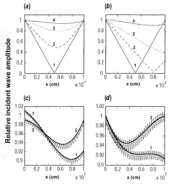
Figure 3: The $x$-dependencies of relative amplitudes $|S_{20}(x)/S_{10}|$ of the incident wave inside the holographic grating with the same parameters as for figure 2 ($\epsilon_{2}=5$, $\epsilon_{g}=5\times 10^{-3}$, $L=10\mu$m, $\theta_{10}=\pi/4$, $\lambda(\mathrm{vacuum})=1\mu$m). (a, b) $\Delta\epsilon_{1}=\epsilon_{1}-\epsilon_{2}\neq 0$ and $\Delta\epsilon_{3}=\epsilon_{3}-\epsilon_{2}=0$ (variations of the mean permittivity only at the front boundary). Curves 1: $\Delta\epsilon_{1}=0$, $\Delta\epsilon_{3}=0$. Curves 2, 3, 4: (a) $\Delta\epsilon_{1}=-10^{-4}$, $-10^{-3}$, $-10^{-1}$, respectively; (b) $\Delta\epsilon_{1}=10^{-4}$, $10^{-3}$, $10^{-1}$. (c, d) The approximate (thick solid curves) and rigorous (oscillating thin curves) dependencies of the relative incident wave amplitudes in the same grating but with (c) $\Delta\epsilon_{3}=0$, $\Delta\epsilon_{1}=0.1$ (curves 1) and $\Delta\epsilon_{1}=-0.1$ (curves 2); (d) $\Delta\epsilon_{1}=0$, $\Delta\epsilon_{3}=0.1$ (curves 1) and $\Delta\epsilon_{3}=-0.1$ (curves 2).

Typical approximate dependencies of the normalized amplitude of the incident wave on the $x$-coordinate inside a narrow grating are presented in figures 3(a), (b) for the same structure as figures 2(a), (b), i.e. with $\epsilon_{2}=5$, $\epsilon_{g}=5\times 10^{-3}$, $\lambda=1\mu$m, $\theta_{10}=45^{\circ}$, $L=10\mu$m, and $\Delta\epsilon_{3}=0$ (i.e. there is no variation of the mean permittivity at the rear grating boundary).

If the variation of the mean permittivity at the front boundary $\Delta\epsilon_{1}$ ¡ 0 (i.e. $\epsilon_{1}<\epsilon_{2}$—figure 3(a)), the scattered wave does not carry the energy away from the grating, and energy conservation results in the same magnitudes of the amplitudes of the incident wave at the front ($x=0$) and rear ($x=L$) boundaries (figure 3(a)). If $\Delta\epsilon_{1}>0$ (i.e. $\epsilon_{1}>\epsilon_{2}$—see figure 3(b)), then the scattered wave at $x<0$ is a propagating wave carrying energy away from the grating. As a result, the amplitude of the incident wave at the rear boundary is smaller than at the front boundary (figure 3(b)).

If the mean permittivity varies at the rear boundary, i.e. $\Delta\epsilon_{3}\neq 0$ and $\Delta\epsilon_{1}=0$, then for small variations of the mean permittivity ($\Delta\epsilon_{1,3}\ll\epsilon_{2}$) the approximate dependencies of the incident wave amplitude in narrow gratings are approximately the same as for the case with $\Delta\epsilon_{3}=0$ and $\Delta\epsilon_{1}\neq 0$ (figures 3(a), (b)). The smaller the grating width, the more accurate is this statement. Note, however, that this is not true for large variations of the mean permittivity $\Delta\epsilon_{1,3}\approx\epsilon_{2}$, for which reflection of the incident wave from the front boundary becomes noticeable.

If $\Delta\epsilon_{1}$ and/or $\Delta\epsilon_{3}$ are positive in a narrow grating with $L<L_{c}$, then it is possible to choose optimal values of $\Delta\epsilon_{1,3}\ll\epsilon_{2}$ such that the amplitude of the incident wave at the rear boundary is next to zero. The smaller the grating width, the smaller the amplitude of the incident wave at the rear boundary can be. In this case, almost total conversion of the energy of the incident wave into energy of the scattered wave occurs. This is radically different from the conventional scattering in narrow gratings with small amplitude, where scattering is very inefficient and the scattered wave amplitude is small (as is the energy flow in it).

If $\Delta\epsilon_{3}=0$ and $\Delta\epsilon_{1}\neq 0$, then the rigorous $x$-dependencies of the amplitude of the zeroth diffracted order are practically the same as the corresponding approximate dependencies of the incident wave amplitude (figure 3(c)). The main distinctive feature of the rigorous dependencies is the weak fast oscillations with the period of the order of the wavelength (figure 3(c)). These oscillations are related to boundary scattering of the scattered wave at the grating interface $x=L$ [10]. The wave resulting from this boundary scattering propagates in the negative $x$-direction as if it is a mirror reflected incident wave from this boundary. Therefore, mathematically, the zeroth term in equation (2) includes both the incident wave and the wave caused by the boundary scattering [10]. Interference of these two waves results in a standing wave pattern represented by fast oscillations of amplitude of the zeroth diffracted order. The period of these oscillations, $\lambda/(2\epsilon^{1/2}_{2}\cos\theta_{20})$, is in excellent agreement with the period of oscillations of the rigorous dependencies in figure 3(c).

It is interesting that if variations of the mean permittivity occur at the rear grating boundary, i.e. $\Delta\epsilon_{3}\neq 0$, then the amplitude of oscillations of the rigorous dependencies may be significantly larger (figure 3(d)). Increasing $|\Delta\epsilon_{3}|$ results in increasing amplitude of these oscillations. This is due to reflection of the incident wave from the rear grating boundary with $\Delta\epsilon_{3}\neq 0$. Mathematically, the reflected wave is also included in the zeroth term in equation (2). Its amplitude increases with increasing $|\Delta\epsilon_{3}|$, which results in stronger oscillations of the resultant interference pattern.

It follows that the difference between the approximate and rigorous curves in figure 3(d) can be reduced by including the reflected wave into the approximate analysis. Indeed, the total electric field resulting from the interference of the incident and reflected waves is given as

$$[S_{20}(x)+S_{2r}\exp(-2\mathrm{i}k_{20x}x)]\exp(\mathrm{i}k_{20x}x+\mathrm{i}k_{10y}y-\mathrm{i}\omega t),$$ (9)

where $S_{20}(x)$ is the $x$-dependent amplitude of the incident wave in the grating, and $S_{2r}$ is the amplitude of the wave reflected from the rear grating boundary (as mentioned above, $S_{2r}$ is given by the Fresnel equations for reflection of the incident wave with the amplitude $S_{20}(L)$ from the interface $x=L$). Wave (9) has a periodically varying amplitude (the expression in the square brackets). If we plot the $x$-dependencies of the magnitude of this amplitude for the gratings corresponding to curves 1 and 2 in figure 3(d), the resultant approximate (oscillating) curves will be very close to the rigorous oscillating curves in figure 3(d). (Note that in the rigorous approach the term $S_{2r}\exp(-2\mathrm{i}k_{20x}x)$ is formally included in the amplitude $S_{20}(x)$.)

3.2 Wide gratings

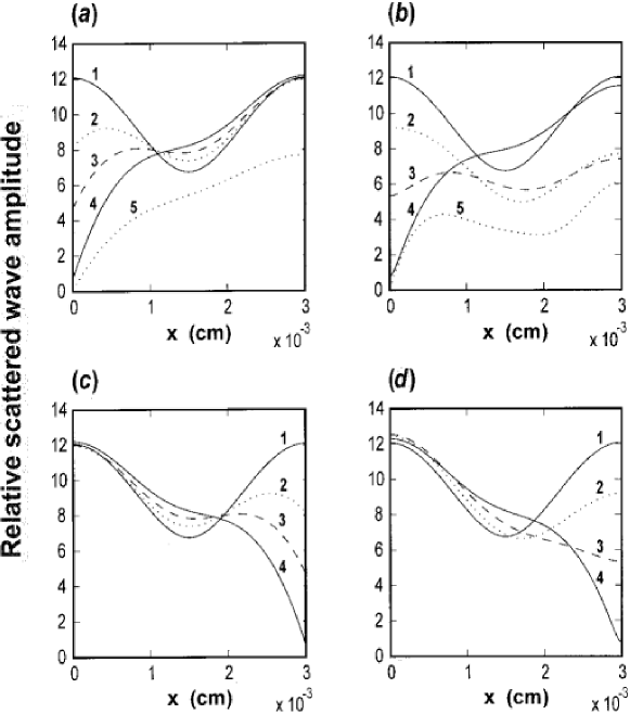
Figure 4: The $x$-dependencies of relative scattered wave amplitudes $|S_{21}(x)/S_{10}|$ inside the holographic grating with the same parameters as for figure 2, but with $L\approx L_{c}\approx 30\mu$m. (a, b) $\Delta\epsilon_{1}\neq 0$ and $\Delta\epsilon_{3}=0$, (c, d) $\Delta\epsilon_{1}=0$ and $\Delta\epsilon_{3}\neq 0$. Curves 1: $\Delta\epsilon_{1}=0$ and $\Delta\epsilon_{3}=0$. Curves 2, 3, 4: (a) $\Delta\epsilon_{1}=-10^{-4}$, $-10^{-3}$, $-10^{-1}$, respectively; (b) $\Delta\epsilon_{1}=10^{-4}$, $10^{-3}$, $10^{-1}$; (c) $\Delta\epsilon_{3}=-10^{-4}$, $-10^{-3}$, $-10^{-1}$; (d) $\Delta\epsilon_{3}=10^{-4}$, $10^{-3}$, $10^{-1}$. Curves 5: (a) $\Delta\epsilon_{1}=-4$, i.e. $\epsilon_{1}=1$ (vacuum in front of the grating), and (b) $\Delta\epsilon_{1}=4.9$ (in this case the angle of incidence $\theta_{10}=45^{\circ}$ is very close to the critical angle $\approx 45.29^{\circ}$ for the interface $x=0$).

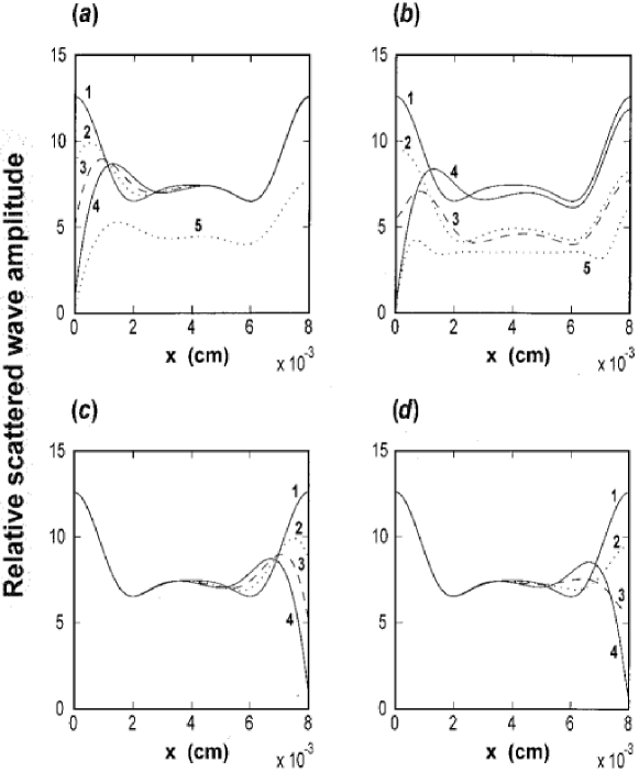
Figure 5: Same as figure 4, but for grating width $L=80\mu\mathrm{m}>L_{c}\approx 30\mu$m.

If the grating width $L\geq L_{c}$, then the pattern of scattering changes significantly. Typical $x$-dependencies of the scattered wave amplitude inside the grating of critical width ($L=L_{c}\approx 30\mu$m) are presented in figure 4. It can be seen that in this case the effect of varying mean permittivity on the scattered wave amplitude tends to be localized in the half of the grating that is adjacent to the boundary at which the variation occurs (figure 4). This tendency becomes much more obvious if we consider EAS in wide gratings, e.g. with $L=80\mu\mathrm{m}>L_{c}\approx 30\mu$m—figure 5.

If the variation of the mean permittivity occurs at the rear boundary (figures 4(c), (d) and 5(c), (d)), then the effect of this variation on the scattered wave amplitude is always localized within the distance $\approx L_{c}/2$ near the rear boundary. Everywhere else in the grating, the scattered wave amplitude is hardly affected by the varying mean permittivity for small and large, positive and negative values of $\Delta\epsilon_{3}$ (figures 4(c), (d) and 5(c), (d)). This is because the diffractional divergence can effectively spread the scattered wave only within distances $\approx L_{c}/2$ [7–9,12], and thus the effects of any perturbations at the rear boundary (e.g. variation of the mean permittivity) can be felt only within these distances (figures 4(c), (d) and 5(c), (d)).

If a variation of the mean permittivity occurs at the front boundary, i.e. $\Delta\epsilon_{1}\neq 0$, then for negative values of $\Delta\epsilon_{1}$ (figures 4(a), 5(a)) the situation is largely the same as in figures 4(c), (d) and 5(c), (d). However, if $|\Delta\epsilon_{1}|$ is large (of the order of $\epsilon_{2}$), then the scattered wave amplitude is affected (reduced) everywhere in the grating—see curves 5 in figures 4(a), 5(a). This is mainly because when $\Delta\epsilon_{1}$ is large and negative, the amplitude of the incident TE wave transmitted through the boundary $x=0$ into the grating is noticeably less than the amplitude of the incident wave in the region $x<0$. This must also result in a reduction of the scattered wave amplitude everywhere in the grating.

If $\Delta\epsilon_{1}>0$ (figures 4(b), 5(b)), then increasing $\Delta\epsilon_{1}$ results in a monotonous decrease of the scattered wave amplitude near the front boundary to about zero (similar to figures 4(a), 5(a)). However, inside the grating (and at the rear boundary) the situation is different. The scattered wave amplitude decreases with increasing $\Delta\epsilon_{1}$ (curves 1–3 in figures 4(b), 5(b)), goes through a minimum, increases back to approximately the same values as for gratings with $\epsilon_{1}=\epsilon_{2}=\epsilon_{3}$ (see curves 1 and 4 in figures 4(b), 5(b)), and then decreases again for large $\Delta\epsilon_{1}$ (curves 5 in figures 4(b), 5(b)).

The more complex behaviour of the curves in figures 4(a), (b) and 5(a), (b) compared to the curves in figures 4(c), (d) and 5(c), (d) is mainly related to the fact that if a perturbation occurs at the front boundary, then the effect of this perturbation can be spread into the grating not only by means of the diffractional divergence of the scattered wave, but also by means of the incident wave that propagates into the grating. At the same time, the effect of perturbations at the rear boundary can be spread into the grating only by means of the diffractional divergence of the scattered wave. Therefore the effect of varying mean permittivity at the front boundary may affect the wave amplitudes everywhere in the grating (figures 4(a), (b) and 5(a), (b)), whereas variations of the mean permittivity at the rear boundary may affect the wave amplitudes only within the distance $\approx L_{c}/2$ from the rear boundary (figures 4(c), (d) and 5(c), (d)).

The noticeable differences between figures 4(a), 5(a) and figures 4(b), 5(b) are due to the fact that if $\Delta\epsilon_{1}>0$ (figures 4(b), 5(b)), then the scattered wave in the region $x<0$ carries the energy away from the grating (see also the discussions of figure 2). The resultant energy losses from the grating can cause noticeable reduction of the scattered wave amplitude in the whole grating (see curves 1–3 in figures 4(b), 5(b)). However, if the variation of the mean permittivity $\Delta\epsilon_{1}$ is sufficiently large, then the amplitude of the scattered wave at the front boundary is small (curves 4 in figures 4(b), 5(b)). As a result, the energy losses drastically reduce, and the scattered wave amplitude inside the grating (not near the front boundary) increases—compare curves 2, 3 and 4 in figures 4(b), 5(b). For a particular value of $\epsilon_{1}$ (in our examples this is $\epsilon_{1}=\epsilon_{1c}=10$), the angle of incidence $\theta_{10}$ (if it is non-zero) becomes equal to the critical angle for the interface $x=0$. In this case, the incident wave in the grating propagates parallel to this interface, i.e. $\theta_{20}=\pi/2$. On the other hand, if the angle of incidence in the grating $\theta_{20}\rightarrow\pi/2$, the amplitude of the scattered wave is strongly reduced [4]. This is the reason for the reduction of the scattered wave amplitudes represented by curves 5 in figures 4(b) and 5(b).

If the mean permittivity varies simultaneous at both the boundaries, then the effect of such variations is roughly the superposition of the effects of separate variations at each of the boundaries. This statement holds better for small variations of mean parameters.

An important general feature of EAS can be seen from the approximate and rigorous analyses of scattering of bulk electromagnetic waves in narrow and wide gratings. Increasing or decreasing wavelength $p$ times with the simultaneous increasing or decreasing grating width $p$ times leaves the amplitudes of the scattered and incident waves unchanged (though scaled to different grating width). For example, EAS of bulk TE waves of $\lambda=2\mu$m in gratings with $L=160\mu$m will be represented by exactly the same curves as in figures 5(a)–(d) with $x/2$ instead of $x$ on the horizontal axis (scaling to the two times larger grating width). The other structural parameters are assumed to be the same as for figure 5.

Similarly, $p$ times increase or decrease of the dielectric permittivity in the structure (including grating amplitude and step-like variations of the mean permittivity) with the simultaneous $p^{1/2}$ times decrease or increase of the grating width also leaves the wave amplitudes unchanged (though again scaled to the different grating width).

4 EAS of guided modes

As has been mentioned in the Introduction, the approximate method of analysis of EAS described is directly applicable to the case of EAS of guided optical modes of arbitrary polarization in gratings with constant mean structural parameters [2,5,6,9,12]. Here, we will see that this is also true for EAS of optical modes guided by a slab with varying mean thickness at the grating boundaries. In this case, the plane of figure 1 is the plane of the slab. One of the boundaries of the slab is periodically corrugated within the strip of width $L$ (figure 1). Thus the thickness of the waveguide inside and outside the grating is given by the equation:

$$h(x_{0})=\left\{\begin{array}[]{l}h_{1},\\ h_{2}+\xi_{g}f(x_{0})\\ h_{3},\end{array},\textrm{for}\right\{\begin{array}[]{l}x<0,\\ 0<x<L,\\ x>L,\end{array}$$ (10)

where $h_{2}$ is the mean thickness of the slab inside the grating region, $h_{1}$ and $h_{3}$ are the slab thicknesses outside the grating, $\xi_{g}$ is the grating amplitude (corrugation amplitude), $f(x_{0})$ is a periodic function with the period $\Lambda$, $\mathrm{max}(|f(x_{0})|)=1$, and the average (over the period) value of $f(x_{0})$ is equal to zero. Dissipation is neglected and all media in contact are isotropic. The variations of the mean slab thickness at the front and rear boundaries are given by $\Delta h_{1}=h_{1}-h_{2}$ and $\Delta h_{3}=h_{3}-h_{2}$ ($\Delta h_{1,3}$ can obviously be either positive or negative).

As in the case of bulk electromagnetic waves in structures described by equation (1), the most interesting case of resonantly strong EAS of guided modes occurs at small grating amplitudes:

$$|\xi_{g}|/\Lambda\ll 1.$$ (11)

In this case, the approximate theory (based on the two-wave approximation and the scalar theory of diffraction) is again expected to give highly accurate results (see [9,10,12]).

Using speculations similar to those in section 2, one comes to the conclusion that equations (4) also describe EAS of guided modes in gratings with varying mean thickness at the grating boundaries. However, the coupling coefficients $\Gamma_{0}$ and $\Gamma_{1}$ are obviously different from those for bulk TE waves and are determined in the approximate theories of conventional Bragg scattering in corrugation gratings with grooves parallel to the grating boundaries [22–25]. The wave numbers for the incident and scattered modes (e.g. $k_{11}$, $k_{21}$, $k_{20}$, etc.) are determined by the dispersion equation for the corresponding slab modes. The effective dielectric permittivities corresponding to these modes can be introduced by the equations: $\epsilon_{21\mathrm{eff}}=k_{21}c/\omega)^{2}$, $\epsilon_{20\mathrm{eff}}=k_{20}c/\omega)^{2}$, etc.

Similarly to bulk electromagnetic waves experiencing reflection and refraction at the grating boundaries with non-zero $\Delta\epsilon_{1,3}$, guided incident and scattered modes also interact with the step-like variations of the mean thickness of the slab. For example, interaction of the incident mode with a step-like variation of $h$ at the front boundary results in generation of other guided modes in the slab and bulk electromagnetic waves outside the slab [22–26]. In the approximate theory, however, all these waves do not contribute to scattering in the grating, except for one guided mode for which the Bragg condition is satisfied. Therefore, the situation is similar to the approximate theory of EAS of bulk electromagnetic waves in section 2. For example, from consideration of the interaction of the incident mode with the front boundary (by means of the mode matching theory [22–26]), one can determine the amplitudes and the directions of propagation of the resulting bulk and guided waves, and then regard the guided mode with the amplitude $S_{200}$, the angle of propagation $\theta_{20}$, and the wave vector $\mathbf{k}_{20}$ that satisfies the Bragg condition as the incident wave at $x=0$ in the grating (inside the grating, the amplitude of this wave is $S_{20}(x)$).

It follows that equations (4)–(7) are directly applicable to the analysis of EAS of guided modes in corrugation gratings with step-like variations of the mean slab thickness. In this case, however, appropriate equations have to be used for the coupling coefficients, wave numbers, and it is assumed that $S_{20}$, $S_{21}$, $A_{0}$, and $B_{0}$ are components of the electric or magnetic field in the incident and scattered modes. Note also that this approach is valid for both TE and TM guided modes.

Interaction of the scattered wave with step-like variations of the mean thickness at the grating boundaries also results in the generation of bulk and guided waves. This means that boundary conditions (8) (except for the first one) have to be modified in order to include these bulk and guided waves. This can again be done in the general case in the same way as in the mode matching theory [22–26].

However, manufacturing gratings with small amplitude usually results in small variations of the mean thickness of the slab. Adsorption and deposition of thin films on the slab surface (e.g. in the region $x<0$) also results in only small variations of mean slab parameters (thickness or effective dielectric permittivity). Therefore, small variations of mean slab thickness are of most importance from the viewpoint of experimental observation and applications of EAS.

The analysis of EAS in such structures does not require the general approaches of the mode matching theory and can be carried out by means of approximate boundary conditions similar to (8). This is because if $\Delta h_{1,3}\ll h_{2}$, then reflection and transformation of modes at such small stepwise variations of the mean slab thickness can be neglected. It can be seen that in this case, for TM modes, the boundary conditions at the grating boundaries $x=0$ and $x=L$ can be written as

$$S_{20}|_{x=0}=S_{200},E_{21z}|_{x=0}=E_{11z}|_{x=0},(\mathrm{d}E_{21z}/\mathrm{d}x)_{x=0}=(\mathrm{d}E_{11z}/\mathrm{d}x)_{x=0},$$

$$E_{21z}|_{x=L}=E_{31z}|_{x=L},(\mathrm{d}E_{21z}/\mathrm{d}x)_{x=L}=(\mathrm{d}E_{31z}/\mathrm{d}x)_{x=L}.$$ (12)

For TE modes, the $z$-components of the electric fields should be replaced by the $z$-components of the magnetic field. $S_{20}$ is the amplitude of one of the components of the electric (or magnetic) field in the incident TM (or TE) mode inside the grating region (note that if $\Delta h_{1}\ll h_{2}$, then $S_{200}\approx S_{10}$—the amplitude of the incident wave in the region $x<0$, and $\theta_{20}\approx\theta_{10}$). The incident and scattered modes are assumed to be of arbitrary order.

It can be seen that equations (12) are exactly the same as equations (8) with the only difference that the $z$-components of the electric or magnetic fields in equations (12) replace the total electric field in equations (8).

When using the boundary conditions (12), it is convenient to use effective dielectric permittivities for the scattered modes: $\epsilon_{11\mathrm{eff}}=k_{11}c/\omega)^{2}$, $\epsilon_{21\mathrm{eff}}=k_{21}c/\omega)^{2}$, and $\epsilon_{31\mathrm{eff}}=k_{31}c/\omega)^{2}$ in front, inside and behind the grating, respectively. In this case, step-like variations of the mean slab thickness at the grating boundaries are related to the corresponding step-like variations of the mean effective permittivities. For example, for the front boundary:

$$\Delta\epsilon_{11\mathrm{eff}}=\epsilon_{11\mathrm{eff}}-\epsilon_{21\mathrm{eff}}\approx\frac{2k_{21}c^{2}}{\omega^{2}}\left(\frac{\mathrm{d}k_{21}}{\mathrm{d}h}\right)_{h=h_{2}}\Delta h_{1}.$$ (13)

As mentioned above, this formula (and the similar one for the rear boundary) is correct only if $\Delta h_{1,3}\ll h_{2}$. Note that we do not have to consider step-like variations of the effective permittivity for the incident wave. These variations can be neglected since for $\Delta h_{1,3}\ll h_{2}$ we have: $S_{10}\approx S_{200}$ and $\theta_{20}\approx\theta_{10}$ (and similar for the rear boundary), i.e. interaction of the incident mode with the grating boundaries can be neglected. (Note that, though being small, $\Delta\epsilon_{11\mathrm{eff}}$ cannot be neglected owing to its significant effect on the diffractional divergence of the scattered wave.)

For example, consider EAS of an incident TE zeroth (TE0) mode into the scattered TE0 mode in the structure: vacuum–GaAs slab (permittivity 12.25)–AlGaAs substrate (permittivity 10.24); the mean slab thickness within the grating region $h_{2}=6\times 10^{-5}$cm, $\theta_{20}\approx\theta_{10}=\pi/4$ (for small values of $\Delta h_{1}\ll h_{2}$), the wavelength in vacuum $\lambda=1.5\times 10^{-4}$cm, the corrugation is assumed to be sinusoidal, i.e. $f(x_{0})=\sin(x_{0})$, and the effective permittivity $\epsilon_{21\mathrm{eff}}\approx 11.48$. The period of the corrugation, determined by the Bragg condition, is $\Lambda\approx 0.579\mu$m. The wavelength of the guided TE₀ mode in this structure is $0.42\mu$m, which is 92% of the wavelength ($0.45\mu$m) in the grating used for figures 2–5. Therefore, according to the general tendency discussed at the end of section 3, in order to get the same dependencies for the guided modes as in figures 2–5, we need to use the gratings of widths $0.92L$ (where $L$ is the width in figures 2–5), and the step-like variations of the slab thickness determined by equation (13) with

$$\Delta\epsilon_{1,3\mathrm{eff}}\approx\frac{\Delta\epsilon_{1,3}}{\epsilon_{2}}\epsilon_{21\mathrm{eff}},$$ (14)

where $\epsilon_{2}=5$ and $\Delta\epsilon_{1,3}$ are the variations of the mean permittivity in figures 2–5. In this case, the corrugation amplitude can be chosen ($\xi_{g}\approx 2\times 10^{-6}$cm) so that the $x$-dependencies of amplitudes of the scattered and incident slab modes in the grating are exactly the same as those given by figures 2–5 with the replacement of $x$ by $x/0.92$ on the horizontal axis (scaling to the new grating width).

It can be seen from equations (13) and (14) that the variations of the mean dielectric permittivity in figures 2–5 $\Delta\epsilon_{1,3}=10^{-5}$, $10^{-4}$, $10^{-3}$, $10^{-1}$ correspond to $\Delta h_{1,3}\approx 1.3\times 10^{-3}$nm, $0.13$ nm, $1.3$ nm, 130 nm in the considered guiding structure. Thus variations of the mean thickness of $\approx 0.1$ monolayer may result in noticeable variations of the scattered wave amplitude in the structure—see curve 2 in figures 2(b), (d). Obviously, on the one hand, this is a significant complication to the experimental observation and application of EAS of guided modes. On the other hand, this demonstrates a very high sensitivity of EAS to conditions on slab interfaces, which may open up excellent opportunities for the design of highly sensitive optical sensors (such as adsorption sensors, sensors of dielectric permittivity, etc.).

If the high sensitivity of EAS to varying mean structural parameters is not desirable, then one should use wide gratings, where the effect of varying mean parameters at the grating boundaries is noticeable only within a half of the critical distance—see figures 4 and 5. Also, use of larger grating amplitudes results in reduction of the sensitivity of EAS to varying mean parameters. Another option is to use grazing-angle scattering (GAS) [12] rather than EAS, where the amplitude of the scattered wave may be especially large at the middle of the grating but not at its boundaries. There is also a possibility of compensating (at least partial) for varying mean parameters by choosing the angle of scattering so that the scattered wave outside the grating propagates parallel to the grating [27].

Another option for the reduction of the high sensitivity of EAS for guided modes is to use slabs with larger thickness $h$, and permittivity that is closer to the permittivities of the surrounding media. For example, in the structure with a polymer slab (dielectric permittivity 2.56) on a silica substrate (dielectric permittivity 2.22), $h=2\mu$m, $\lambda=1.4\mu$m, $L=20\mu$m, and grating amplitude $\xi_{g}=3.3\times 10^{-5}$cm we have: $\epsilon_{21\mathrm{eff}}=2.49$, and the equivalent structure for bulk waves (having the same dependencies of the wave amplitudes) must have $\epsilon_{2}=\epsilon_{21\mathrm{eff}}$, same $\lambda$ and $L$, and $\epsilon_{g}=7\times 10^{-3}$. In this case, $\Delta\epsilon_{1}=10^{-4}$ in the equivalent structure corresponds to a variation in the mean thickness $\Delta h_{1}\approx 1.8$ nm. These variations of the permittivity or thickness result in $\approx 15$% reduction of the scattered wave amplitude from $\approx 8S_{200}$ to $\approx 6.8S_{200}$ at the front grating boundary $x=0$. Recall that a similar 15% variation of the scattered wave amplitude in the GaAs waveguide with $L=9.2\mu$m, $h=0.6\mu$m, and $\xi_{g}=2\times 10^{-6}$cm is achieved at a much smaller value of $\Delta h_{1}\approx 1.3\times 10^{-2}$nm—compare curves 1 and 2 in figure 2(b).

Finally, it is important to note that in the case of EAS of surface waves (e.g. surface acoustic waves, or surface electromagnetic waves) in corrugation gratings, the problem with varying mean parameters hardly exists. This is because in this case the step-like variation of the mean level of the substrate surface inside and outside the grating does not affect the length of the wave vector (or the wavelength) of the surface waves. Only if, for example, outside the grating we have additional layers on the surface, may the mean propagation parameters change and the above-mentioned effects occur. Thus a surface wave sensor based on EAS in periodic groove arrays is especially easy to design.

5 Conclusions

This paper has demonstrated yet another unique feature of scattering of optical waves in extremely asymmetrical geometry—the unusual sensitivity of the incident and scattered wave amplitudes to small stepwise variations of mean structural parameters (e.g. mean dielectric permittivity or mean waveguide thickness). This effect has no analogies in conventional Bragg scattering. It has been explained by the high sensitivity of diffractional divergence to small variations of mean structural parameters across an optical beam.

Two distinct typical patterns of scattering have been described for gratings that are narrower and wider than a grating of critical width $L_{c}$ [7–9] (half of $L_{c}$ is equal to the distance within which the scattered wave can be spread across the grating by means of the diffractional divergence, before it is re-scattered by the grating [7–9]). In particular, it has been shown that in narrow gratings (with $L<L_{c}$), varying mean permittivity at either of the boundaries strongly affects the scattered wave amplitude everywhere in the structure, whereas in wide gratings (with $L>L_{c}$), the effect of varying mean parameters is usually (but not always) significant only within the distance $L_{c}/2$ from the boundaries.

The analysis has been carried out by means of approximate and rigorous methods, showing a very good agreement between them for the most interesting cases of strong EAS in gratings with small amplitude.

The analysis of EAS of guided modes has revealed especially high sensitivity of scattered wave amplitudes to small variations of the mean slab thickness. This is mainly due to strong dispersion of guided modes, i.e. strong dependence of their wave numbers on slab thickness. This sensitivity may, on the one hand, present a complication for experimental observation of EAS, and on the other hand, be very useful for the application of EAS in the design of highly sensitive sensors and measurement techniques. Several options for dealing with this possible experimental complication are discussed.

References

1. Kishino, S., Noda, A., and Kohra, K., 1972, J. Phys. Soc. Japan., 33, 158.

2. Bakhturin, M. P., Chernozatonskii, L. A., and Gramotnev, D. K., 1995, Appl. Opt., 34, 2692.

3. Gramotnev, D. K., 1995, Phys. Lett. A, 200, 184.

4. Gramotnev, D. K., 1997, J. Physics D, 30, 2056.

5. Gramotnev, D. K., 1997, Opt. Lett., 22, 1053.

6. Gramotnev, D. K., and Pile, D. F. P., 1999, App. Opt., 38, 2440.

7. Gramotnev, D. K., and Pile, D. F. P., 1999, Phys. Lett. A, 253, 309.

8. Gramotnev, D. K., and Nieminen, T. A., 1999, J. Opt. A: Pure Appl. Opt., 1, 635.

9. Gramotnev, D. K., and Pile, D. F. P., 2000, Opt. Quantum Electron., 32, 1097.

10. Nieminen, T. A., and Gramotnev, D. K., 2001, Opt. Commun., 189, 175.

11. Gramotnev, D. K., 2000, Frequency response of extremely asymmetrical scattering of electromagnetic waves in periodic gratings, 2000 Diffractive Optics and Micro-Optics (DOMO-2000), Quebec City, Canada, pp.165–167.

12. Gramotnev, D. K., 2001, Opt. Quantum Electron., 33, 253.

13. Moharam, M. G., Grann, E. B., Pommet, D. A., and Gaylord, T. K., 1995, J. Opt. Soc. Am., A12, 1068.

14. Moharam, M. G., Pommet, D. A., Grann, E. B., and Gaylord, T. K., 1995, J. Opt. Soc. Am., A12, 1077.

15. Chateau, N., and Hugonin, J. P., 1994, J. Opt. Soc. Am., A11, 1321.

16. Li, L., 1996, J. Opt. Soc. Am., A13, 1024.

17. Liu, J., Chen, R. T., Davies, B. M., and Li, L., 1990, Appl. Op., 38, 6981.

18. Li, L., Chandezon, J., Granet, G., and Plumey, J. P., 1999, Appl. Opt., 38, 304.

19. Akhmediev, N., and Ankiwicz, A., 1997, Solitons, Non-linear Pulses and Beams (London: Chapman & Hall).

20. Gramotnev, D. K., and Pile, D. F. P., 2001, J. Opt. A: Pure Appl. Opt., 3, 103.

21. Gaylord, T. K., and Moharam, M. G., 1985, Proc. IEEE, 73, 894.

22. Popov, E., and Mashev, L., 1985, Opt. Acta, 32, 265.

23. Biehlig, W., Hehl, K., Langbein, U., and Leberer, F., 1986, Opt. Quantum Electron., 18, 219.

24. Biehlig W., 1986, Opt. Quantum Electron., 18, 229.

25. Shigesawa, H., and Tsuji, M., 1986, IEEE Trans. Microwave Theory Tech., MMT-34, 205.

26. Borsboom, P. P., and Frankena, H. J., 1995, J. Opt. Soc. Am., A12, 1134.

27. Gramotnev, D. K., and Andres, Ch., Grazing-angle scattering of waves in infinitely wide periodic gratings, 2002, (unpublished).