Relativistic correlation correction to the binding energies of the ground configuration of Beryllium-like, Neon-like, Magnesium-like and Argon-like ions

Abstract

Total electronic correlation correction to the binding energies of the isoelectronic series of Beryllium, Neon, Magnesium and Argon, are calculated in the framework of relativistic multiconfiguration Dirac-Fock method. Convergence of the correlation energies is studied as the active set of orbitals is increased. The Breit interaction is treated fully self-consistently. The final results can be used in the accurately determination of atomic masses from highly charged ions data obtained in Penning-trap experiments.

1 Introduction

The determination of an accurate value for the fine structure constant $\alpha$ and of accurate mass values has received latelly special attention due to recent works on highly ionized atoms using Penning traps 645 ; 833 ; 832 . The relative uncertainties of such experimental results can vary from $10^{-7}$ to $10^{-10}$, depending on the handled ionic species, on the lifetime of the nucleus and on the experimental apparatus.

When calculating the atomic mass from the experimentally observed ion mass with this technique, one has to account for the mass $qm_{e}$ of the $q$ removed electrons and their atomic binding energy $E_{B}$. Therefore, the mass of atom X is given by

$$m_{\text{X}}=m_{\text{X}^{q+}}+qm_{e}-\frac{E_{B}}{c^{2}}$$ (1)

The influence of the binding energy uncertainties on the mass determination depends on the specific atom, and increases with the $Z$ value. For example, in the Cs mass determination, an uncertainty of about 10 eV in the calculated K-, Ar-, and Cl-like Cs ions binding energies  671 originates an uncertainty of the order of $10^{-11}$ in the mass determination  645 .

This means that for the largest uncertainties a simple relativistic calculated value, in the framework of the Dirac-Fock (DF) approach, is more than sufficient. However, if the experimental apparatus provides values with an accuracy that approaches the lower side of the mentioned interval, one has to perform more sofisticated theoretical calculations, such as the ones that use the Multi-Configuration Dirac-Fock (MCDF) model which includes electronic correlation, in order to achieve a comparable accuracy in the binding energy determination.

In this article we provide accurate correlation contribution to the binding energy for the Be-like, Ne-like, Mg-like and Ar-like systems for atomic numbers up to $Z=95$. We also study self-energy screening effects. The correlation energies provided here are designed to correct the Dirac-Fock results of Ref. risp2003 for relativistic correlation effects. In that work, Dirac-Fock energies for all iso-electronic series with 3 to 105 electrons, and all atomic numbers between 3 and 118 are provided, using the same electron-electron interaction operator described in Sec. 2. In Sec. 2 we give the principle of the calculations, namely a brief description of the MCDF method used in these calculations and the enumeration of the radiative corrections included. In Sec. 3 we present the results of calculations and the conclusions are given in Sec. 4. All numerical results presented here are evaluated with values of the fundamental constants from the 1998 adjustment 765 .

2 Calculations

To perform theoretical relativistic calculations in atomic systems with more than one electron, the Brown and Ravenhall problem 231 , related to the existence of the $E<-mc^{2}$ continuum, must be taken in account. To overcome this situation, Sucher 229 sugested that a proper form of the electron-electron interaction with projection operators onto the $E>mc^{2}$ continuum must be used, leading to the so called no-pair Hamiltonian,

$${\cal H}^{\mbox{{\tiny no pair}}}=\sum_{i=1}^{N}{\cal H}_{D}(r_{i})+\sum_{i<j}{\cal V}(|\bm{r}_{i}-\bm{r}_{j}|),$$ (2)

where ${\cal H}_{D}$ is the one electron Dirac operator and ${\cal V}_{ij}=\Lambda^{++}_{ij}V_{ij}\Lambda^{++}_{ij}$ is an operator representing the electron-electron interaction of order $\alpha$ 47 ; 230 . Here $\Lambda^{++}_{ij}=\Lambda^{+}_{i}\Lambda^{+}_{j}$ is an operator projecting onto the positive energy Dirac eigenstates to avoid introducing unwanted pair creation effects. There is no explicit expression for $\Lambda^{++}$, except at the Pauli approximation 864 . The elimination of the spurious contributions from the $E<-mc^{2}$ continuum in the MCDF method 47 is achieved by solving the MCDF radial differential equations on a finite basis set and keeping in the basis set expansion only the solutions whose eigenvalues are greater than $-mc^{2}$ in order to remove the negative continuum. The basis set used is made of B-Splines. The method of Ref. 47 suffers however from limitations and inaccuracies due to limitations of the B-Spine basis. When the number of occupied orbitals is increased, these numerical errors prevent convergence. In that case we had to calculate without projecting. However this problem is not very severe, as the role of the negative energy continuum becomes less and less important when the number of electrons increases. In the 4 isoelectronic series studied here, only the Be-like sequence was sensistive to the presence of the projection operator even at relatively low $Z$. In the other series, only the case with $Z=95$ involving the $6h$ shell would have required it. In the latter case convergence was impossible whether a projection operator was used or not.

The electron-electron interaction operator $V_{ij}$ is gauge dependent, and is represented in the Coulomb gauge and in atomic units, by:

$$V_{ij} = \,\,\,\,\frac{1}{r_{ij}}$$ (3c)

$$-\frac{\bm{\alpha}_{i}\cdot\bm{\alpha}_{j}}{r_{ij}}$$

$$-\frac{\bm{\alpha}_{i}\cdot\bm{\alpha}_{j}}{r_{ij}}[\cos\left(\frac{\omega_{ij}r_{ij}}{c}\right)-1]$$

$$+c^{2}(\bm{\alpha}_{i}\cdot\bm{\nabla}_{i})(\bm{\alpha}_{j}\cdot\bm{\nabla}_{j})\frac{\cos\left(\frac{\omega_{ij}r_{ij}}{c}\right)-1}{\omega_{ij}^{2}r_{ij}},$$

where $r_{ij}=\left|\bm{r}_{i}-\bm{r}_{j}\right|$ is the inter-electronic distance, $\omega_{ij}$ is the energy of the exchanged photon between the two electrons, $\bm{\alpha}_{i}$ are the Dirac matrices and $c=1/\alpha$ is the speed of light. The term (3c) represents the Coulomb interaction, the second one (3c) is the Gaunt (magnetic) interaction, and the last two terms (3c) stand for the retardation operator 845 ; 846 . In the above expression the $\bm{\nabla}$ operators act only on $r_{ij}$ and not on the following wave functions. By a series expansion in powers of $\omega_{ij}r_{ij}/c\ll 1$ of the operators in expressions (3c) and (3c) one obtains the Breit interaction, which includes the leading retardation contribution of order $\alpha^{2}$. The Breit interaction is the sum of the Gaunt interaction (3c) and of the Breit retardation

$$B^{\mbox{\scriptsize{R}}}_{ij}={\frac{\bm{\alpha}_{i}\cdot\bm{\alpha}_{j}}{2r_{ij}}}-\frac{\left(\bm{\alpha}_{i}\cdot\bm{r}_{ij}\right)\left(\bm{\alpha}_{j}\cdot\bm{r}_{ij}\right)}{2r_{ij}^{3}}.$$ (4)

In the present calculation the electron-electron interaction is described by the sum of the Coulomb and the Breit interaction. The remaining contributions due to the difference between Eqs. (3c) and (4) were treated only as a first order perturbation.

2.1 Dirac-Fock method

A first approach in relativistic atomic calculations is obtained through the relativistic counterpart of the non-relativistic Hartree-Fock (HF) method, the Dirac-Fock method. The principles underlying this method are virtually the same as those of the non-relativistic one. In the DF method the electrons are treated in the independent-particle approximation, and their wave functions are evaluated in the Coulomb field of the nucleus and the spherically-averaged field from the electrons. A natural improvement of the method is the generalization of the electronic field to include other contributions, such as the Breit interaction.

The major limitation of this method lies in the fact that it makes use of the spherically-averaged field of the electrons and not of the local field; i.e., it does not take into account electronic correlation.

2.2 Multiconfiguration Dirac-Fock method

To account for electron correlation not present at the DF level, one may add to the initial DF configuration, configurations with the same parity and total angular momentum, involving unoccupied (virtual) orbitals This is the principle of the Multiconfiguration Dirac-Fock method.

The total energy of an atom, or ion, is the eigenvalue of the following equation:

$${\cal H}^{\mbox{{\tiny no pair}}}\Psi_{\Pi,J,M}(\ldots,\bm{r}_{i},\ldots)=E_{\Pi,J,M}\Psi_{\Pi,J,M}(\ldots,\bm{r}_{i},\ldots),$$ (5)

where $\Pi$ is the parity, $J^{2}$ is the total angular momentum with eigenvalue $J$ and its projection on the $z$ axis $J_{z}$, with eigenvalue $M$. The MCDF method is defined by the particular choice of the total wave function $\Psi_{\Pi,J,M}(...,\bm{r}_{i},...)$ as a linear combination of configuration state functions (CSF):

$$\mid\Psi_{\Pi,J,M}\rangle=\sum_{\nu}c_{\nu}\mid\nu\Pi JM\rangle.$$ (6)

The CSF are chosen as eigenfunctions of $\Pi$, $J^{2}$, and $J_{z}$. The label $\nu$ stands for all other numbers (principal quantum number, coupling, …) necessary to define unambiguously the CSF. For a $N$-electron system, the CSF is a linear combination of Slater determinants

$$\mid\nu\Pi JM\rangle=\sum_{i}d_{i}\left|\begin{array}[]{ccc}\Phi_{1}^{i}(r_{1})&\cdots&\Phi_{N}^{i}(r_{1})\\ \vdots&\ddots&\vdots\\ \Phi_{1}^{i}(r_{N})&\cdots&\Phi_{N}^{i}(r_{N})\end{array}\right|,$$ (7)

where the $\Phi$-s are the one-electron wave functions. In the relativistic case, they are the Dirac four-component spinors:

$$\Phi_{n\kappa\mu}(\bm{r})=\frac{1}{r}\left[\begin{array}[]{c}P_{n\kappa}(r)\chi_{\kappa\mu}(\theta,\phi)\\ iQ_{n\kappa}(r)\chi_{-\kappa\mu}(\theta,\phi)\end{array}\right]$$ (8)

where $\chi_{\kappa\mu}(\theta,\phi)$ is a two component Pauli spherical spinors 78 and $P_{n\kappa}(r)$ and $Q_{n\kappa}(r)$ are the large and the small radial components of the wave function, respectively. The functions $P_{n\kappa}(r)$, $Q_{n\kappa}(r)$ are the solutions of coupled integro-differential equations obtained by minimizing Eq. (5) with respect to each radial wave function. The coefficients $d_{i}$ are determined numericaly by requiring that each CSF is an eigenstate of $J^{2}$ and $J_{z}$, while the coefficients $c_{\nu}$ are determined by diagonalization of the Hamiltonian matrix (for more details see, e.g., Refs. 31 ; 78 ; 282 ).

The numerical methods as described in Refs. 47 ; 282 , enabled the full relaxation of all orbitals included and the complete self-consistent treatment of the Breit interaction, i.e., in both the Hamiltonian matrix used for the determination of the mixing coefficients $c_{\nu}$ in Eq. (6) and of the differential equations used to obtain the radial wave functions. To our knowledge, this is a unique feature of the MCDF code we used, since others only include the Breit contribution in the determination of the mixing coefficients (see, e.g., 329 ).

2.3 Radiative Corrections

The present work is intended to provide correlation energies to complement the results listed in Ref. risp2003 . Radiative corrections are already included in Ref. risp2003 . However, we give here a discussion of the self-energy screening correction, in view of a recent work iam2001 , to compare the uncertainty due to approximate evaluation of multi-electron QED corrections and those due to correlation.

The radiative corrections due to the electron-nucleus interaction, namely the self-energy and the vacuum polarization, which are not included in the Hamiltonian discussed in the previous sections, can be obtained using various approximations. Our evaluation, mostly identical to the one in Ref. risp2003 is described as follows.

One-electron self-energy is evaluated using the one-electron results by Mohr and coworkers 115 ; 114 ; 116 for several $(n,\ell)$, and corrected for finite nuclear size 117 . Self-energy screening and vacuum polarization are treated with the approximate method developed by Indelicato and coworkers  58 ; 56 ; 53 ; 847 . These methods yield results in close agreement with more sophisticated methods based on QED  242 ; 263 ; 288 . More recently a QED calculation of the self-energy screening correction between electrons of quantum numbers $n\leq 2$, $\ell=0,1$, has been published iam2001 , which allows to evaluate the self-energy screening in the ground state of 2- to 10-electron ions. In the present work we use these results to evalute the self-energy screening in Be-like and Ne-like ions.

3 Results and Discussion

3.1 Correlation

To obtain the uncorrelated energy we start from a Dirac-Fock calculation, with Breit interaction included self-consistently. This correspond to the case in which the expansion (6) has only one term in the present work since we study ions with only closed shells.

The active variational space size is increased by enabling all single and double excitations from all occupied shells to all virtual orbitals up to a maximum $n$ and $\ell=n-1$ including the effect of the electron-electron interaction to all-orders (see  671 for further details). For example, in the Be-like ion case both the $1s$ and $2s$ occupied orbitals are excited up to $2p$, then up to $3d$, $4f$, $5g$, and $6h$. We can then compare the difference between successive correlation energies obtained in this way, to assess the convergence of the calculation. When calculating correlation corrections to the binding energy it is obviously important to excite the inner shells, as the correlation contribution to the most bound electrons provides the largest contribution to the total correlation energy. However this leads to very large number of configuration when the number of occupied orbitals is large.

In the present calculations we used a virtual space spanned by all singly and doubly-excited configurations. For the single excitations we excluded the configurations in which the electron was excited to an orbital of the same $\kappa$ as the initial orbital (Brillouin orbitals). In the present case, where there is only one $jj$ configuration in the reference state, those excitations do not change the total energy, according to the Brillouin theorem (see, e.g., bauche:72 ; godefroid:1987:brillouin ; froese:00 ). That would not be true in cases with open shells in the reference state as it was recently demonstrated ild2005 . The choice of single and double substitutions is due to computation reasons and is justified by the overwhelming weight of these contributions.

For all iso-electronic sequences considered here, we included all configurations with active orbitals up to $6h$, except sometimes for the neutral case or for $Z=95$, for which convergence problems were encountered. The generation of the multiconfiguration expansions was automatically within the mdfgme code. The latest version can generate all single and double excitations from all the occupied levels in a given configuration to a given maximum value of the principal and angular quantum numbers. The number of configurations used to excite all possible pairs of electrons to the higher virtual orbitals considered is shown in Table 1. This table shows the rapid increase of the number of configurations with the number of electrons.

Table 1: Number of $jj$ configurations within a given virtual space identified by the correlation orbital with the highest $(n,\ell)$ quantum numbers.

	$2p$	$3d$	$4f$	$5g$	$6h$
Be-like	8	38	104	218	392
Ne-like		84	386	1007	2039
Mg-like		84	486	1359	2838
Ar-like		56	712	2422	5505

In Table 2 we provide a detailed study of the contributions to the correlation energy of Be-like ions for $Z$ in the range $4\leq Z\leq 95$. We compare several cases. In the first case the Coulomb correlation energy is evaluated using only the operator given by Eq. (3c). In the second case, the wavefunctions are evaluated with the same operator in the SCF process, and used to calculate the mean-value of the Breit operator (4). Finally, we include the Breit operator both in the differential equation used to evaluate the wavefunction (Breit SC) and in the Hamiltonian matrix. For high-$Z$, relativistic corrections dominate the correlation energy, which no longer behaves as $A+B/Z+...$, as is expected in a non-relativistic approximation. The contribution from the Breit operator represents 34 % of the Coulomb contribution. It is thus clear that any calculation claiming sub-eV accuracy must include the effect of Breit correlation. Obviously higher-order QED effects, not obtainable by an Hamiltonian-based formalism, can have a similar order of magnitude.

Table 2: Details of the results for the correlation energy of Be-like ions as a function of the operator used in the evaluation of the wavefunction and of the size of the active space (see explanations in the text). “all $\to n\ell$”: double excitations from all occupied orbitals to all shells up to $n\ell$ are included.

	Coulomb Correlation, Coulomb SC
$Z$	$2s^{2}+2^{p}2$	all $\to 2p$	all $\to 3d$	all $\to 4f$	all $\to 5g$
4	-1.192	-1.192	-2.172	-2.306	-2.392
10	-3.323	-3.328	-4.364	-4.586	-4.688
15	-4.867	-4.876	-5.939	-6.171	-6.274
18	-5.710	-5.720	-6.796	-7.031	-7.136
25	-7.340	-7.353	-8.457	-8.700	-8.807
35	-8.755	-8.774	-9.921	-10.176	-10.286
45	-9.399	-9.427	-10.618	-10.887	-11.000
55	-9.741	-9.778	-11.016	-11.299	-11.417
65	-10.013	-10.057	-11.351	-11.649	-11.775
75	-10.273	-10.321	-11.689	-12.007	-12.142
85	-10.556	-10.607	-12.078	-12.421	-12.568
95	-11.042	-11.094	-12.717	-13.095	-13.257
	Total Correlation, Coulomb SC
$Z$	$2s^{2}+2^{p}2$	all $\to 2p$	all $\to 3d$	all $\to 4f$	all $\to 5g$
4	-1.192	-1.192	-2.176	-2.310	-2.396
10	-3.325	-3.330	-4.390	-4.617	-4.722
15	-4.873	-4.882	-6.003	-6.246	-6.357
18	-5.720	-5.731	-6.890	-7.142	-7.257
25	-7.367	-7.382	-8.648	-8.923	-9.048
35	-8.813	-8.835	-10.298	-10.612	-10.753
45	-9.480	-9.513	-11.217	-11.575	-11.734
55	-9.829	-9.874	-11.863	-12.269	-12.445
65	-10.103	-10.159	-12.483	-12.933	-13.147
75	-10.381	-10.446	-13.172	-13.678	-13.926
85	-10.720	-10.794	-14.011	-14.585	-14.878
95	-11.308	-11.392	-15.236	-15.897	-16.245
	Total Correlation, Breit SC
$Z$	$2s^{2}+2^{p}2$	all $\to 2p$	all $\to 3d$	all $\to 4f$	all $\to 5g$	all $\to 6h$
4	-1.192	-1.192	-2.176	-2.310	-2.396
10	-3.325	-3.330	-4.406	-4.616	-4.723	-4.759
15	-4.873	-4.882	-6.004	-6.245	-6.360	-6.380
18	-5.721	-5.732	-6.887	-7.136	-7.254	-7.303
25	-7.367	-7.382	-8.658	-8.936	-9.066	-9.122
35	-8.814	-8.836	-10.334	-10.659	-10.811	-10.879
45	-9.483	-9.517	-11.308	-11.692	-11.870	-11.951
55	-9.836	-9.884	-12.048	-12.502	-12.710	-12.805
65	-10.116	-10.179	-12.813	-13.353	-13.594	-13.707
75	-10.402	-10.481	-13.712	-14.355	-14.638	-14.771
85	-10.750	-10.847	-14.843	-15.618	-15.951	-16.109
95	-11.349	-11.473	-16.467	-17.415	-17.812

In Tables 3 to 5 we list the correlation energy for the Ne-, Mg- and Ar-like sequence with fully self-consistent Breit interaction, for different sizes of the active space. Double excitations from all occupied orbitals to all possible shells up to $3d$, $4f$, $5g$ and $6h$ are included, except when it was not possible to reach convergence.

Table 3: Calculated total correlation energy for the Ne sequence, for different sets of SCF. “all $\to n\ell$”: double excitations from all occupied orbitals to all shells up to $n\ell$ are included. Results with Breit self consistent included in the calculation.

$Z$	all $\to 3d$	all $\to 4f$	all $\to 5g$	all $\to 6h$
10	-5.911	-8.306	-9.339	-9.709
15	-5.989	-8.712	-9.838	-10.280
25	-6.374	-9.310	-10.494	-10.967
35	-6.710	-9.850	-11.099	-11.609
45	-7.074	-10.482	-11.816	-12.372
55	-7.515	-11.269	-12.710	-13.322
65	-8.067	-12.260	-13.833	-14.511
75	-8.752	-13.375	-15.247	-16.007
85	-9.772	-15.119	-17.056	-17.916
95	-11.160	-17.231	-19.429	-20.415
105	-13.061	-20.129	-22.689

Table 4: Details of the results for the correlation energy of Mg-like ions as a function of the operator used in the evaluation of the wavefunction and of the size of the active space (see explanations in the text). “all $\to n\ell$”: double excitations from all occupied orbitals to all shells up to $n\ell$ are included.

	Coulomb Correlation, Coulomb SC
$Z$	all $\to 3d$	all $\to 4f$	all $\to 5g$	all $\to 6h$
12	-3.372	-7.823	-9.741
20	-5.211	-9.724	-11.809	-12.640
25	-5.878	-10.470	-12.582	-13.442
35	-6.852	-11.588	-13.768	-14.638
45	-7.477	-12.349	-14.597	-15.477
55	-7.845	-12.810	-15.185	-16.071
65	-8.063	-13.179	-15.642	-16.541
75	-8.220	-13.596	-16.081	-17.001
85	-8.378	-14.006	-16.598	-17.550
95	-8.597	-14.560	-17.307	-18.305
	Total Correlation, Coulomb SC
$Z$	all $\to 3d$	all $\to 4f$	all $\to 5g$	all $\to 6h$
12	-3.379	-7.836	-9.786
20	-5.241	-9.792	-11.971	-12.833
25	-5.932	-10.598	-12.855	-13.768
35	-6.977	-11.891	-14.351	-15.338
45	-7.702	-12.902	-15.614	-16.693
55	-8.200	-13.668	-16.753	-17.933
65	-8.580	-14.424	-17.879	-19.172
75	-8.934	-15.374	-19.112	-20.523
85	-9.328	-16.401	-20.572	-22.117
95	-9.833	-17.718	-22.422
	Total Correlation, Breit SC
$Z$	all $\to 3d$	all $\to 4f$	all $\to 5g$	all $\to 6h$
12	-3.379	-7.864	-9.734
20	-5.241	-9.793	-11.972	-12.830
25	-5.932	-10.599	-12.857	-13.762
35	-6.976	-11.899	-14.356	-15.325
45	-7.701	-12.932	-15.611	-16.676
55	-8.198	-13.808	-16.799	-17.939
65	-8.577	-14.677	-18.009	-19.247
75	-8.928	-15.670	-19.375	-20.772
85	-9.319	-16.939	-21.062
95	-9.826	-18.695	-23.244

Table 5: Details of the results for the correlation energy of Ar-like ions as a function of the size of the active space (see explanations in the text). “all $\to n\ell$”: double excitations from all occupied orbitals to all shells up to $n\ell$ are included. Results with Breit self consistent included in the calculation.

$Z$	all $\to 3d$	all $\to 4f$	all $\to 5g$	all $\to 6h$
18	-3.258	-10.462	-13.886
20	-4.003	-11.700	-15.203	-17.557
25	-5.441	-13.851	-17.755	-19.994
35	-7.689	-16.982	-21.292	-23.578
45	-9.482	-19.441	-24.093	-26.472
55	-10.844	-21.455	-26.486	-28.985
65	-11.746	-23.077	-28.564	-31.213
75	-12.197	-24.380	-30.426	-33.257
85	-12.254	-25.499	-32.229	-35.278
95	-12.002	-26.644	-34.207

In Fig. 1 to 4 we present the evolution of the correlation energy $E_{c}$ (in eV), defined by the diference between the total binding energy obtained with the MCDF method and the one obtained by the DF method, with the increase of the virtual space for each isoelectronic series studied. We notice, as expected, a decrease of the energy with the increase of the atomic number and the increase of the number of virtual orbitals.

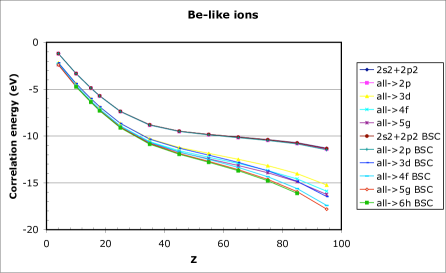
Figure 1: Evolution of the correlation energy $E_{c}$ (in eV) for Be-like ions, defined by the diference between the total binding energy obtained with the MCDF method and the one obtained by the DF method, with the increase of virtual space.

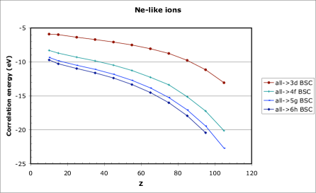
Figure 2: Evolution of the correlation energy $E_{c}$ (in eV) for Ne-like ions, defined by the diference between the total binding energy obtained with the MCDF method and the one obtained by the DF method, with the increase of virtual space.

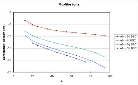
Figure 3: Evolution of the correlation energy $E_{c}$ (in eV) for Mg-like ions, defined by the diference between the total binding energy obtained with the MCDF method and the one obtained by the DF method, with the increase of virtual space.

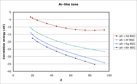
Figure 4: Evolution of the correlation energy $E_{c}$ (in eV) for Ar-like ions, defined by the diference between the total binding energy obtained with the MCDF method and the one obtained by the DF method, with the increase of virtual space.

An inspection of Fig. 1 to 4 and of Tables 3 to 5 gives a clear indication of the importance of including a specific shell in the calculation for the value of the correlation, i.e., if a new curve, corresponding to the inclusion of a specific shell, is close to the previous curve, obtained through the inclusion of shells of lower principal quantum number, it means that we have included the major part of the correlation in the energy calculation. We can also see the effect of including or not the Breit interaction in the SCF process. Our calculation is accurate within a few 0.01 eV for low-$Z$ Be-like ions up to 0.15 eV at high-$Z$. For Ne-like ions, we find respectively 0.4 eV and 1 eV, for Mg-like ions we find 0.9 and 1.4 eV, and for Ar-like ions these numbers are 2.3 and 3 eV. It is thus clear that the maximum value of $n$ and $\ell$ one should go to reach uniform accuracy increases with the number of electrons. However the uncertainty due to this limitation of our calculation is probably negligible compare to neglected QED corrections like the contribution from negative energy continuum, box diagram and two-loop QED corrections.

In order to provide values for arbitrary atomic numbers within each isoelectronic series we have fitted polynomials to the best correlation curves. The equations for these fits are given in Table 6.

Table 6: Fit to the ground state total correlation energy $\Delta E$ of the Be, Ne, Mg and Ar isoelectronic sequences, with correlation orbitals up to $6h$

Series	Fit
Be	$\Delta E=1.421329\times 10^{-7}Z^{4}-7.019909\times 10^{-5}Z^{3}+9.159169\times 10^{-3}Z^{2}-5.474933\times 10^{-1}Z-7.191674\times 10^{-2}$
Ne	$\Delta E=5.523943\times 10^{-8}Z^{4}-2.760868\times 10^{-5}Z^{3}+2.214132\times 10^{-3}Z^{2}-1.324244\times 10^{-1}Z-8.627745$
Mg	$\Delta E=-2.156149\times 10^{-8}Z^{4}-1.529410\times 10^{-5}Z^{3}+2.928077\times 10^{-3}Z^{2}-2.903759\times 10^{-1}Z-8.078404$
Ar	$\Delta E=5.696195\times 10^{-7}Z^{4}-1.529548\times 10^{-4}Z^{3}+1.589991\times 10^{-2}Z^{2}-9.710181\times 10^{-1}Z-3.406304$

We present in Table 7 the different terms contributing to the total atomic binding energy of Be-like ions with $Z=4$, 45 and 85, to illustrate their relative importance.

Table 7: Contributions to the atomic binding energy for for ions of different $Z$ in the Beryllium isoelectronic serie (in eV).

	Z=4	Z=45	Z=85
Coulomb	-398.91260	-68961.32493	-272463.59996
Magnetic	0.01430	39.84888	310.21457
Retardation (order $\omega^{2}$)	0.00105	-0.58860	-6.10695
Higher-order retardation ($>\omega^{2}$)	0.00000	0.00000	0.00000
Hydrogenlike self-energy	0.01310	62.62419	610.43890
Self-energy screening	-0.00291	-1.76962	-13.44919
Vacuum polarization (Uheling) $\alpha(Z\alpha)$	-0.00039	-7.46054	-139.37727
Electronic correction to Uheling	0.00004	0.03290	0.33323
Vacuum polarization $\alpha(Z\alpha)^{3}$	0.00000	0.12368	6.14067
Vac. Pol. (Källèn & Sabry) $\alpha^{2}(Z\alpha)$	0.00000	-0.06042	-1.07200
Recoil	0.00000	-0.00805	-0.06221
Correlation	-2.39600	-11.95100	-16.10900
Total Energy	-401.28341	-68880.53351	-271712.6492

3.2 Self-energy screening

In Table 8 we compare the self-energy screening correction evaluated by the use of Ref. iam2001 and by the Welton method. Direct evaluation of the screened self-energy diagram using Ref. iam2001 , includes relaxation only at the one-photon exchange level. The Welton method include relaxation at the Dirac-Fock or MCDF level. In the case of Be-like ions we also performed a calculation including intra-shell correlation to have an estimate of the effect of correlation on the self-energy screening. The change due to the method is much larger than the effect of even strong intra-shell correlation. The difference between the two evaluations of the self-energy screening can reach $\approx 2$ eV at Z=95.

Table 8: Comparison of the screened self-energy contribution in Be-like and Ne-like ions obtained by different methods.

	Be-like				Ne-like
	Ref. iam2001		Welton model		Ref. iam2001	Welton model
Z	$2s^{2}$	$2s^{2}+2p^{2}$	$2s^{2}$	$2s^{2}+2p^{2}$
4	-0.004	-0.004	-0.003	-0.003
10	-0.047	-0.046	-0.036	-0.035	-0.081	-0.050
15	-0.132	-0.129	-0.104	-0.101	-0.229	-0.155
25	-0.466	-0.458	-0.384	-0.375	-0.835	-0.614
35	-1.066	-1.053	-0.917	-0.903	-1.973	-1.519
45	-1.995	-1.976	-1.801	-1.783	-3.825	-3.060
55	-3.349	-3.323	-3.190	-3.165	-6.659	-5.530
65	-5.282	-5.248	-5.317	-5.279	-10.888	-9.388
75	-8.054	-8.012	-8.562	-8.499	-17.178	-15.373
85	-12.130	-12.080	-13.546	-13.439	-26.659	-24.737
95	-19.176	-19.109	-21.347	-21.162	-41.114	-39.721

4 Conclusions

We have presented relativistic calculations of the correlation contribution to the total binding energies for ions of the Beryllium, Neon, Magnesium and Argon isoelectronic series. We have shown that accurate results can be achieved if excitations to all shells up to the $n=6$ shell are included.We have also compared two different methods for the evaluation of the self-energy screening. Combined with the results of Ref. risp2003 our results will provide binding energies with enough accuracy for all ion trap mass measurements to come, involving ions with the isolelectronic sequences considered here.

References

- (1) C. Carlberg, T. Fritioff, I. Bergström, Phys. Rev. Lett. 83, 4506 (1999).
- (2) D. Beck, F. Ames, G. Audi, G. Bollen, F. Herfurth, H. J. Kluge, A. Kohl, M. Konig, D. Lunney, I. Martel, R. B. Moore, H. R. Hartmann, E. Schark, S. Schwarz, M. d. S. Simon, J. Szerypo, Eur. Phys. J. A 8, 307 (2000).
- (3) G. Douysset, T. Fritioff, C. Carlberg, I. Bergström, M. Bjorkhage, Phys. Rev. Lett. 86, 4259 (2001).
- (4) G. C. Rodrigues, M. A. Ourdane, J. Bieroń, P. Indelicato, E. Lindroth, Phys. Rev. A 63, 012510, 012510 (2001).
- (5) G. C. Rodrigues, P. Indelicato, J. P. Santos, P. Patté, At. Data Nucl. Data Tables 86, 117 (2004).
- (6) P. J. Mohr B. N. Taylor, Rev. Mod. Phys. 72, 351 (2000).
- (7) G. E. Brown D. E. Ravenhall, Proc. R. Soc. London, Ser. A 208, 552 (1951).
- (8) J. Sucher, Phys. Rev. A 22, 348 (1980).
- (9) P. Indelicato, Phys. Rev. A 51, 1132 (1995).
- (10) M. H. Mittleman, Phys. Rev. A 24, 1167 (1981).
- (11) E. Lindroth, Phys. Rev. A 37, 316 (1988).
- (12) S. A. Blundell, P. J. Mohr, W. R. Johnson, J. Sapirstein, Phys. Rev. A 48, 2615 (1993).
- (13) I. Lindgren, H. Persson, S. Salomonson, L. Labzowsky, Phys. Rev. A 51, 1167 (1995).
- (14) I. P. Grant, Adv. Phys. 19, 747 (1970).
- (15) N. Bessis, G. Bessis, J.-P. Desclaux, J. Phys. 31, C4 (1970).
- (16) J. P. Desclaux, in Methods and Techniques in Computational Chemistry (STEF, Cagliary, 1993), Vol. A.
- (17) K. G. Dyall, I. P. Grant, C. T. Johnson, F. A. Parpia, E. P. Plummer, Comp. Phys. Commun. 55, 425 (1989).
- (18) P. Indelicato P. J. Mohr, Phys. Rev. A 63, 052507 (2001).
- (19) P. J. Mohr, Phys. Rev. A 26, 2338 (1982).
- (20) P. J. Mohr Y.-K. Kim, Phys. Rev. A 45, 2727 (1992).
- (21) P. J. Mohr, Phys. Rev. A 46, 4421 (1992).
- (22) P. J. Mohr G. Soff, Phys. Rev. Lett. 70, 158 (1993).
- (23) P. Indelicato, O. Gorceix, J. P. Desclaux, J. Phys. B 20, 651 (1987).
- (24) P. Indelicato J. P. Desclaux, Phys. Rev. A 42, 5139 (1990).
- (25) P. Indelicato E. Lindroth, Phys. Rev. A 46, 2426 (1992).
- (26) P. Indelicato, S. Boucard, E. Lindroth, Eur. Phys. J. D 3, 29 (1998).
- (27) P. Indelicato P. J. Mohr, Theor. Chim. Acta 80, 207 (1991).
- (28) S. A. Blundell, Phys. Rev. A 46, 3762 (1992).
- (29) S. A. Blundell, Phys. Scr. T46, 144 (1993).
- (30) J. Bauche M. Klapisch, J. Phys. B: At. Mol. Phys. 5, 29 (1972).
- (31) M. Godefroid, J. Lievin, J. Y. Met, J. Phys. B: At. Mol. Phys. 20, 3283 (1987).
- (32) C. F. Fischer, T. Brage, P.Jönsson, Computational Atomic Structure (Institute of Physics Publishing, Bristol, 2000).
- (33) P. Indelicato, E. Lindroth, J. P. Desclaux, Phys. Rev. Lett. 94, 013002 (2005).