Spectral energy dynamics in magnetohydrodynamic turbulence

Abstract

Spectral direct numerical simulations of incompressible MHD turbulence at a resolution of up to $1024^{3}$ collocation points are presented for a statistically isotropic system as well as for a setup with an imposed strong mean magnetic field. The spectra of residual energy, $E_{k}^{\mathrm{R}}=|E_{k}^{\mathrm{M}}-E_{k}^{\mathrm{K}}|$, and total energy, $E_{k}=E^{\mathrm{K}}_{k}+E^{\mathrm{M}}_{k}$, are observed to scale self-similarly in the inertial range as $E_{k}^{\mathrm{R}}\sim k^{-7/3}$, $E_{k}\sim k^{-5/3}$ (isotropic case) and $E^{\mathrm{R}}_{k_{\perp}}\sim k_{\perp}^{-2}$, $E_{k_{\perp}}\sim k_{\perp}^{-3/2}$ (anisotropic case, perpendicular to the mean field direction). A model of dynamic equilibrium between kinetic and magnetic energy, based on the corresponding evolution equations of the eddy-damped quasi-normal Markovian (EDQNM) closure approximation, explains the findings. The assumed interplay of turbulent dynamo and Alfvén effect yields $E_{k}^{\mathrm{R}}\sim kE^{2}_{k}$ which is confirmed by the simulations.

The nonlinear behavior of turbulent plasmas gives rise to a variety of dynamical effects such as self-organization of magnetic confinement configurations in laboratory experiments Ortolani and Schnack (1993), generation of stellar magnetic fields Zeldovich et al. (1983) or structure formation in the interstellar medium Biskamp (2003). The understanding of these phenomena is incomplete as the same is true for many inherent properties of the underlying turbulence.

Large-scale low-frequency plasma turbulence is treated in the magnetohydrodynamic (MHD) approximation describing the medium as a viscous and electrically resistive magnetofluid neglecting additional kinetic effects. Incompressiblity of the flow is assumed for the sake of simplicity. In this setting the nature of the turbulent energy cascade is a central and still debated issue with different phenomenologies being proposed Kolmogorov (1991); Iroshnikov (1964); Kraichnan (1965); Sridhar and Goldreich (1994); Goldreich and Sridhar (1997) (cf. Müller and Biskamp (2002) for a review). The associated spectral dynamics of kinetic and magnetic energy, in spite of its comparable importance, has received less attention (as an exception see Grappin et al. (1983)).

This Letter reports a spectral relation between residual and total energy, $E_{k}^{\mathrm{R}}=|E_{k}^{\mathrm{M}}-E_{k}^{\mathrm{K}}|$ and $E_{k}=E^{\mathrm{K}}_{k}+E^{\mathrm{M}}_{k}$ respectively, as well as the influence of an imposed mean magnetic field on the spectra. The proposed physical picture, which is confirmed by accompanying direct numerical simulations, embraces two-dimensional MHD turbulence, globally isotropic three-dimensional systems as well as turbulence permeated by a strong mean magnetic field.

In the following reference is made to two high-resolution pseudospectral direct numerical simulations of incompressible MHD turbulence which we regard as paradigms for isotropic (I) and anisotropic (II) MHD turbulence. The dimensionless MHD equations

$$\partial_{t}{\bm{\omega}} = \nabla\times\left[{\bm{v}}\times{\bm{\omega}}-{\bm{b}}\times\left(\nabla\times{\bm{b}}\right)\right]+\mu\Delta{\bm{\omega}}$$ (1)

$$\partial_{t}{\bm{b}} = \nabla\times\left({\bm{v}}\times{\bm{b}}\right)+\eta\Delta{\bm{b}}$$ (2)

$$\nabla\cdot{\bm{v}} = \nabla\cdot{\bm{b}}=0\,.$$ (3)

are solved in a $2\pi$-periodic cube with spherical mode truncation to reduce numerical aliasing errors Vincent and Meneguzzi (1991). The equations include the flow vorticity, ${\bm{\omega}}=\nabla\times{\bm{v}}$, the magnetic field expressed in Alfvén speed units, ${\bm{b}}$, as well as dimensionless viscosity, $\mu$, and resistivity, $\eta$. In simulation II forcing is applied by freezing the largest spatial scales of velocity and magnetic field.

Simulation I evolves globally isotropic freely decaying turbulence represented by $1024^{3}$ Fourier modes. The initial fields are smooth with random phases and fluctuation amplitudes following $\exp(-k^{2}/(2k_{0}^{2}))$ with $k_{0}=4$. Total kinetic and magnetic energy are initially equal with $E^{\textrm{K}}=E^{\textrm{M}}=0.5$. The ratio $E^{\textrm{K}}/E^{\textrm{M}}$ decreases in time taking on values of $0.28-0.23$ in the period considered (cf. Biskamp and Müller (1999)). The ratio of kinetic and magnetic energy dissipation rate, $\varepsilon^{K}/\varepsilon^{M}$, with $\mu=\eta=1\times 10^{-4}$ also decreases during turbulence decay from $0.7$ to about $0.6$, the difference in dissipation rates reflecting the imbalance of the related energies. The Reynolds number Re$=(E^{\mathrm{K}})E/(\mu\varepsilon^{\mathrm{total}})$ at $t=6$ is about $2700$ and slightly diminishes during the run. Magnetic, $H^{\mathrm{M}}=\frac{1}{2}\int_{\mathrm{V}}\mathrm{d}\mathrm{V}{\bm{a}}\cdot{\bm{b}}$, ${\bm{b}}=\nabla\times{\bm{a}}$, and cross helicity, $H^{\mathrm{C}}=\frac{1}{2}\int_{\mathrm{V}}\mathrm{d}\mathrm{V}{\bm{v}}\cdot{\bm{b}}$ , are negligible with $H^{\mathrm{C}}$ showing a dynamically unimportant increase from 0.03 to 0.07 during the simulation. The run covers 9 eddy turnover times defined as the time required to reach the maximum of dissipation from $t=0$. The large-scale rms magnetic field decays from initially 0.7 to 0.3.

Case II is a $1024^{2}\times 256$ forced turbulence simulation with an imposed constant mean magnetic field of strength $b_{0}=5$ in units of the large-scale rms magnetic field $b_{\mathrm{rms}}\simeq v_{\mathrm{rms}}\simeq 1$. The forcing, which keeps the ratio of fluctuations to mean field approximately constant, is implemented by freezing modes with $k\leq k_{f}=2$. The simulation with $\mu=\eta=9\times 10^{-5}$ has been brought into quasi-equilibrium over 20 eddy-turnover times at a resolution of $512^{2}\times 256$ and spans about 5 eddy turnover times of quasi-stationary turbulence with $1024^{2}\times 256$ Fourier modes and Re$\approx$$2300$ (based on field perpendicular fluctuations). Kinetic and magnetic energy as well as the ratio $E^{\mathrm{K}}/E^{\mathrm{M}}$ are approximately unity with a slight excess of $E^{\mathrm{M}}$. Perpendicular to the imposed field, large-scale magnetic fluctuations with $b_{\mathrm{rms}}\simeq 0.4$ are observed. Correspondingly, $\varepsilon^{K}/\varepsilon^{M}\simeq 0.95$ during the simulation. The system has relaxed to $H^{\mathrm{C}}\simeq 0.15$ with a fluctuation level of about 30% and $H^{\mathrm{M}}\simeq 0.2H^{\textrm{M}}_{\textrm{Max}}$ with $H^{\textrm{M}}_{\textrm{Max}}\sim E^{\mathrm{M}}/k_{f}$.

Fourier-space-angle integrated spectra of total, magnetic, and kinetic energy for case I are shown in Fig. 1.

Figure 1: Total (solid), kinetic (dashed), and magnetic (dotted) energy spectra in $1024^{3}$ case I simulation (normalized, time-averaged and compensated). Dash-dotted line: $k^{-3/2}$ scaling.

To neutralize secular changes as a consequence of turbulence decay, amplitude normalization is used assuming a Kolmogorov total energy spectrum, $E_{k}\rightarrow E_{k}/(\varepsilon\mu^{5})$, $\varepsilon=-\partial_{t}E$, with wavenumbers given in inverse multiples of the associated dissipation length, $\ell_{\mathrm{D}}\sim(\mu^{3}/\varepsilon)^{1/4}$. The quasi-stationary normalized spectra are time averaged over the period of self-similar decay, $t=6-8.9$. As in previous numerical work Müller and Biskamp (2000); Haugen et al. (2004) and also observed in solar wind measurements Leamon et al. (1998); Goldstein and Roberts (1999), Kolmogorov scaling applies for the total energy in the well-developed inertial range, $0.01\lesssim k\lesssim 0.1$. However, here the remarkable growth of excess magnetic energy with decreasing wavenumber is of interest. Qualitatively similar behavior is observed with large scale forcing exerted on the system. We note that no pile-up of energy is seen at the dissipative fall-off contrary to other high-resolution simulations Haugen et al. (2004); Kaneda et al. (2003). Apart from different numerical techniques and physical models this difference might be due to the limited simulation period at highest resolution namely 5 Haugen et al. (2004) and 4.3 Kaneda et al. (2003) large-eddy-turnover times. Depending on initial conditions the energy spectrum at $1024^{3}$-resolution is still transient at that time.

In case II, pictured in Fig. 2,

Figure 2: Field-perpendicular total (solid), kinetic (dashed), and magnetic (dotted) energy spectra (normalized, time-averaged, and compensated) in $1024^{2}\times 256$ case II simulation with $b_{0}=5$. Dash-dotted curve: high-k part of field-parallel total energy spectrum. Inset: perpendicular total energy spectrum for resolutions of $512^{2}$ (dash-dotted) to $1024^{2}$ (solid).

strong anisotropy is generated due to turbulence depletion along the mean magnetic field, ${\bm{b}}_{0}$, (cf. also Müller et al. (2003); Kinney and McWilliams (1998); Oughton et al. (1998); Grappin (1986); Shebalin et al. (1983)). This is visible when comparing the normalized and time-averaged field-perpendicular one-dimensional spectrum, $E_{k_{\perp}}=\int\int\mathrm{d}k_{1}\mathrm{d}k_{2}E(k_{\perp},k_{1},k_{2})$ (solid line) with the field-parallel spectrum, defined correspondingly and adumbrated by the dash-dotted line in Fig. 2. The fixed $k_{\perp}$-axis is chosen arbitrarily in the $k_{1}$-$k_{2}$-plane perpendicular to ${\bm{b}}_{0}$ where fluctuations are nearly isotropic. For the strong $b_{0}$ chosen here, field-parallel and -perpendicular energy spectra do not differ notably from the ones found by considering the direction of the local magnetic field as done e.g. in Müller et al. (2003); Cho et al. (2002). The field-parallel dissipation length is larger than in field-perpendicular directions because of the stiffness of magnetic field lines. The numerical resolution in the parallel direction can, therefore, be reduced.

While there is no discernible inertial range in the parallel spectrum, its perpendicular counterpart exhibits an interval with Iroshnikov-Kraichnan scaling, $E_{k_{\perp}}\sim k_{\perp}^{-3/2}$ (Note that due to identical energy scales in Figs. 1 and 2 the absolute difference between Kolmogorov and Iroshnikov-Kraichnan scaling is the same as in Fig.1). This is in contradiction to the anisotropic cascade phenomenology of Goldreich and Sridhar for strong turbulence predicting $E_{k_{\perp}}\sim k_{\perp}^{-5/3}$ Goldreich and Sridhar (1997) and with numerical studies claiming to support the GS picture Cho and Vishniac (2000); Cho et al. (2002). However, the strength of ${\bm{b}}_{0}$ in these simulations is of the order of the turbulent fluctuations and consequently much weaker than for the anisotropic system considered here. We note that indication for field-perpendicular IK scaling has been obtained in earlier simulations at lower resolution using a high-order hyperviscosity and with a stronger mean component, $b_{0}/b\sim 3\times 10^{2}$ Maron and Goldreich (2001). The authors of the aforementioned paper, however, are unsure whether they observe a numerical artefact or physical behavior.

The strongly disparate spectral extent of field-parallel and -perpendicular fluctuations suggests that Alfvén waves propagating along the mean field do not have a significant influence on the perpendicular energy spectrum (in the sense of Goldreich-Sridhar, cf. also Kinney and McWilliams (1998)). Instead, the strong ${\bm{b_{0}}}$ constrains turbulence to quasi-two-dimensional field-perpendicular planes as is well known and has been shown for this particular system Müller et al. (2003).

Another intriguing feature of system II is that $E^{\mathrm{K}}_{k}\simeq E^{\mathrm{M}}_{k}$ with only slight dominance of $E^{\mathrm{M}}$ (cf. Fig. 2) in contrast to the growing excess of spectral magnetic energy with increasing spatial scale for case I. Since both states are dynamically stable against externally imposed perturbations (as has been verified numerically), they presumably represent equilibria between two competing nonlinear processes: field-line deformation by turbulent motions on the spectrally local time scale $\tau_{\mathrm{NL}}\sim\ell/v_{\ell}\sim\left(k^{3}E^{\mathrm{K}}_{k}\right)^{-1/2}$ leading to magnetic field amplification (turbulent small-scale dynamo) and energy equipartition by shear Alfvén waves with the characteristic time $\tau_{\mathrm{A}}\sim\ell/b_{0}\sim(kb_{0})^{-1}$ (Alfvén effect). The conjecture can be verified via the EDQNM closure approximation Orszag (1970) which yields evolution equations for kinetic and magnetic energy spectra Pouquet et al. (1976) by including a phenomenological eddy-damping term for third-order moments. The spectral evolution equation for the signed residual energy, $E^{\mathrm{R}}=E^{\text{M}}-E^{\text{K}}$, in the case of negligible cross helicity reads Grappin, U. Frisch, J. Léorat und A. Pouquet (1982):

$$\left(\partial_{t}+\left(\mu+\eta\right)k^{2}\right)E^{\mathrm{R}}_{k} =\int_{\triangle}\text{d}p\text{d}q\Theta_{kpq}\left(T^{\mathrm{R}}_{\mathrm{res}}+T^{\mathrm{R}}_{\mathrm{crs}}+T^{\mathrm{R}}_{\mathrm{Dyn}}\right)$$ (4)

with the spectral energy flux contributions

$$T^{\mathrm{R}}_{\mathrm{res}} =m_{kpq}\frac{k^{2}}{p}E^{\mathrm{R}}_{p}E^{\mathrm{R}}_{q}+r_{kpq}\frac{p^{2}}{q}E^{\mathrm{R}}_{q}E^{\mathrm{R}}_{k}\,,$$

$$T^{\mathrm{R}}_{\mathrm{crs}} =-m_{kpq}pE_{q}E^{\mathrm{R}}_{k}-t_{kpq}pE^{\mathrm{R}}_{q}E_{k}\,,$$

$$T^{\mathrm{R}}_{\mathrm{Dyn}} =\frac{s_{kpq}}{k}\left(k^{2}E_{p}E_{q}-p^{2}E_{q}E_{k}\right).$$

The geometric coefficients $m_{kpq}$, $r_{kpq}$, $s_{kpq}$, $t_{kpq}$, a consequence of the solenoidality constraints (3), are given in Grappin, U. Frisch, J. Léorat und A. Pouquet (1982). The ‘$\triangle$’ restricts integration to wave vectors ${\bm{k}}$, ${\bm{p}}$, ${\bm{q}}$ which form a triangle, i.e. to a domain in the $p$-$q$ plane which is defined by $q=|{\bm{p}}+{\bm{k}}|$. The time $\Theta_{kpq}$ is characteristic of the eddy damping of the nonlinear energy flux involving wave numbers $k$, $p$, and $q$. It is defined phenomenologically but its particular form does not play a role in the following arguments.

Local triad interactions with $k\sim p\sim q$ are dominating the hydrodynamic turbulent energy cascade and lead to Kolmogorov scaling of the associated spectrum (cf., for example, Lesieur (1997)). In contrast, the nonlinear interaction of Alfvén waves includes non-local triads with, e.g., $k\ll p\sim q$. In this case a simplified version of equation (4) can be derived:

$$\partial_{t}E^{\mathrm{R}}_{k} =-\Gamma_{k}kE_{k}^{\mathrm{R}}\equiv T^{\mathrm{R}}_{\mathrm{Alf}},$$ (5)

with $\Gamma_{k}=\frac{4}{3}k\int_{0}^{ak}\text{d}q\Theta_{kpq}E_{q}^{\mathrm{M}}$ Pouquet et al. (1976) $\sim kE^{M}\Theta$.

It is now assumed that the right hand side of (4) can be written as $T^{\mathrm{R}}_{\mathrm{Alf}}+T^{\mathrm{R}}_{\mathrm{Dyn}}$ Grappin et al. (1983). This states that the residual energy is a result of a dynamic equilibrium between turbulent dynamo and Alfvén effect. For stationary conditions and in the inertial range, dimensional analysis of (4) and (5) yields $k^{3}E_{k}^{2}\sim k^{2}E^{\mathrm{M}}E_{k}^{\mathrm{R}}$ which can be re-written as

$$E_{k}^{\mathrm{R}}\sim kE_{k}^{2}\,.$$ (6)

The relaxation time, $\Theta$, appears as a factor on both sides of the relation and, consequently, drops out. We note that with $\tau_{\mathrm{A}}\sim(kb_{0})^{-1}$, where $b_{0}$ is the mean magnetic field carried by the largest eddies, $b_{0}\sim(E^{\mathrm{M}})^{1/2}$, and by re-defining $\tau_{\mathrm{NL}}\sim\ell/(v_{\ell}^{2}+b_{\ell}^{2})^{1/2}\sim(k^{3}E_{k})^{-1/2}$ (for system II all involved quantities are based on field-perpendicular fluctuations) relation (6) can be obtained in the physically more instructive form

$$E_{k}^{\mathrm{R}}\sim\left(\frac{\tau_{\mathrm{A}}}{\tau_{\mathrm{NL}}}\right)^{2}E_{k}\,.$$ (7)

The modification of $\tau_{\mathrm{NL}}$ is motivated by considering that gradients of the Alfvén speed contribute to nonlinear transfer as much as velocity shear (see, e.g., Heyvaerts and Priest (1983)).

For the examined setups relation (7) is consistent with the underlying physical idea of dynamical equilibrium between Alfvén and dynamo effect. At small scales with $k\gg k_{0}$ (for system II: $k_{0}\simeq k_{f}$), Alfvénic interaction always dominates the energy exchange since $\tau_{\mathrm{A}}\ll\tau_{\mathrm{NL}}$ (e.g. at $k=0.3l_{\mathrm{D}}^{-1}$ for system I: $\tau_{\mathrm{A}}\simeq 5\times 10^{-2},\tau_{\mathrm{NL}}\simeq 0.2$, for system II: $\tau_{\mathrm{A}}\simeq 1\times 10^{-2},\tau_{\mathrm{NL}}\simeq 0.1)$ which results in approximate spectral equipartiton of kinetic and magnetic energy. At larger spatial scales the Alfvén effect becomes less efficient in balancing the transformation of kinetic to magnetic energy by the small-scale dynamo with $\tau_{\mathrm{A}}\simeq\tau_{\mathrm{NL}}$ (e.g. at $k=0.01l_{\mathrm{D}}^{-1}$for system I: $\tau_{\mathrm{A}}\simeq 0.9,\tau_{\mathrm{NL}}\simeq 0.8$, at $k=3\times 10^{-3}l_{\mathrm{D}}^{-1}$ for system II: $\tau_{\mathrm{A}}\simeq 1.2,\tau_{\mathrm{NL}}\simeq 0.9)$ allowing larger deviations from equipartition.

An interesting consequence of (6) is that the difference between possible spectral scaling exponents, which is typically small and hard to measure reliably, is enlarged by a factor of two in $E^{\mathrm{R}}_{k}$. Even with the limited Reynolds numbers in today’s simulations such a magnified difference is clearly observable (e.g. dash-dotted lines in Figs. 1 and 3). For system I with Kolmogorov scaling, $E_{k}\sim k^{-5/3}$ (Fig. 1), relation (6) predicts $E^{\mathrm{R}}_{k}\sim k^{-7/3}$ in agreement with the simulation (Fig. 3). In the case of Iroshnikov-Kraichnan behavior, $E_{k_{\perp}}\sim k_{\perp}^{-3/2}$ as realized in system II (Fig. 2), $E^{\mathrm{R}}_{k_{\perp}}\sim k_{\perp}^{-2}$ is obtained. This result is confirmed by the residual energy spectrum shown in Fig. 4 (cf. also Biskamp (1995) for two-dimensional MHD simulations and Grappin et al. (1983) for spectral model calculations).

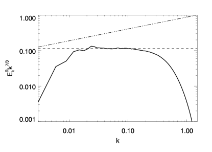
Figure 3: Compensated, space-angle-integrated residual energy spectrum, $E^{\mathrm{R}}_{k}$, for same system as in Fig. 1. Dash-dotted line: $k^{-2}$-scaling.

Figure 4: Compensated field-perpendicular residual energy spectrum for the same system as in Fig. 2.

In summary, based on the structure of the EDQNM closure equations for incompressible MHD a model of the nonlinear spectral interplay between kinetic and magnetic energy is formulated. Throughout the inertial range a quasi-equilibrium of turbulent small-scale dynamo and Alfvén effect leads to the relation, $E^{\mathrm{R}}_{k}\sim kE_{k}^{2}$, linking total and residual energy spectra, in particular $E^{\mathrm{R}}_{k}\sim k^{-7/3}$ for $E_{k}\sim k^{-5/3}$ and $E^{\mathrm{R}}_{k}\sim k^{-2}$ for $E_{k}\sim k^{-3/2}$. Both predictions are confirmed by high-resolution direct numerical simulations, limiting the possible validity of the Goldreich-Sridhar phenomenology to MHD turbulence with moderate mean magnetic fields.