Optimizing at the Ergodic Edge

Abstract

Using a simple, annealed model, some of the key features of the recently introduced extremal optimization heuristic are demonstrated. In particular, it is shown that the dynamics of local search possesses a generic critical point under the variation of its sole parameter, separating phases of too greedy (non-ergodic, jammed) and too random (ergodic) exploration. Comparison of various local search methods within this model suggests that the existence of the critical point is essential for the optimal performance of the heuristic. PACS number(s): 02.60.Pn, 05.40.-a, 64.60.Cn, 75.10.Nr.

I Introduction

Many situations in physics and beyond require the solution of NP-hard optimization problems, for which the typical time needed to ascertain the exact solution apparently grows faster than any power of the system size G+J . Examples in the sciences are the determination of ground states for disordered magnets Dagstuhl04 ; Pal ; Hartmann ; P+Y ; Houdayer99 ; eo_prl or of optimal arrangements of atoms in a compound B+S or a polymer Erzan ; Frauenkorn ; Prellberg . With the advent of ever faster computers, the exact study of such problems has become feasible P+A ; Rinaldi . Yet, with typically exponential complexity of these problems, many questions regarding those systems still are only accessible via approximate, heuristic methods Rayward . Heuristics trade off the certainty of an exact result against finding optimal or near-optimal solutions with high probability in polynomial time. Many of these heuristics have been inspired by physical optimization processes, for instance, simulated annealing Science ; Salamon02 or genetic algorithms Holland .

Extremal optimization (EO) was proposed recently BoPe1 ; Dagstuhl04 , and has been used to treat a variety of combinatorial GECCO ; BoPe2 ; BoPe3 and physical optimization problems eo_prl ; Boettcher03b ; EOSK . Comparative studies with simulated annealing BoPe1 ; GECCO ; EOperc and other Metropolis MRRTT based heuristics D+S ; Boettcher05b have established EO as a successful alternative for the study of NP-hard problems. EO has found a large number of applications, for instance, in pattern recognition MB ; Meshoul03 , signal filtering YomTov , transport problems Sousa04a molecular dynamics simulations Zhou05 , artificial intelligence Menai03a ; Menai03b , social modeling Duch05 , and $3d$ spin glass models D+S ; Wang03 ; Onody03 . There are also a number of studies that have explored basic features of the algorithm eo_jam ; Boettcher05b , extensions Middleton04 ; Sousa03b ; Sousa04b , and rigorous performance properties Heilmann04 ; Hoffmann04 .

In this article, we will use a simple, annealed model of a generic combinatorial optimization problem, introduced in Ref. eo_jam , to compare analytically certain variations of local search with EO, and of Metropolis algorithms such as Simulated Annealing (SA) Science ; Salamon02 . This comparison affirms the notion of “optimization at the ergodic edge” that motivated the $\tau$-EO implementation BoPe1 ; eo_prl . This implementation possesses a single tunable parameter, $\tau$, which separates a phase of “greedy” search from a phase of wide fluctuations, combining both features at the phase transition into an ideal search heuristic for rugged energy landscapes Frauenfelder . The model helps to identify the distinct characteristics of different search heuristics commonly observed in real optimization problems. In particular, revisiting the model with a “jammed” state from Ref. eo_jam proves the existence of the phase transition to be essential for the superiority of EO, at least within a one-parameter class of local search heuristics. At the phase boundary, EO descends sufficiently fast to the ground state with enough fluctuations to escape jams.

This article is organized as follows: In the next section, we introduce the annealed optimization model, followed in Sec. III by a short review of the local search heuristics studied here, in particular, of one-parameter variations of EO and of Metropolis-based search. Then, in Sec. IV we compare our analytical results for each heuristic in the annealed model. In Sec. V we show why versions of EO lacking a phase transition fail to optimize well. We summarize our results and draw some conclusions in Sec. VI.

II Annealed Optimization Model

As described in Ref. eo_jam , we can abstract certain combinatorial optimization problems into a simple, analytically tractable model. To motivate this model we imagine a generic optimization problem as consisting of a number of variables $1\leq i\leq n$, each of which contributes an amount $-\lambda_{i}$ to the overall cost per variable (or energy density) of the system,

$$\epsilon=-\frac{1}{2n}\sum_{i=1}^{n}\lambda_{i}.$$ (1)

(The factor $1/2$ arises because local cost are typically equally shared between neighboring variables.) We call $\lambda_{i}\leq 0$ the “fitness” of the variable, where larger values are better and $\lambda_{i}=0$ is optimal for each variable. Correspondingly, $\epsilon=0$ is the (optimal) ground state of the system. In a realistic problem, variables are correlated such that not all of them could be simultaneously of optimal fitness. But in our annealed model, those correlations are neglected.

A concrete example for the above definitions is provided by a spin glass with the Hamiltonian

$$H=-\sum_{i,j}J_{i,j}\sigma_{i}\sigma_{j}$$ (2)

with some quenched random mix of bonds $J_{i,j}=\in\{-1,0,+1\}$ and spin variables $\sigma_{i}=\pm 1$ eo_prl . With $\lambda_{i}=\sigma_{i}\sum_{j}J_{i,j}\sigma_{j}-\sum_{j}|J_{i,j}|$, counting (minus) the number of violated bonds of each spin $i$ (among its $\alpha_{i}$ non-zero bonds), it is $\epsilon=H/n+\epsilon_{0}$, where $\epsilon_{0}$ is an insignificant constant.

We will consider that each variable $i$ is in one of $\alpha+1$ ($\alpha_{i}=\alpha$ constant) different fitness states $\lambda_{i}$. We can specify occupation numbers $n_{a}$, $0\leq a\leq\alpha$, for each state $a$, and define occupation densities $\rho_{a}=n_{a}/n~{}(a=0,\ldots,\alpha)$. Hence, any local search procedure Rayward with single-variable updates, say, can be cast simply as a set of evolution equations for the $\rho_{a}(t)$, i. e.

$${\dot{\rho}}_{b}=\sum_{a}T_{b,a}Q_{a}.$$ (3)

The $Q_{a}$ are the probabilities that a variable in state $a$ gets updated; any local search process (based on updating a finite number of variables) defines a unique set of $Q_{a}$, as we will see below. The matrix $T_{b,a}$ specifies the net transition to state $b$ given that a variable in state $a$ is updated. This matrix allows us to design arbitrary, albeit annealed, optimization problems. Both, ${\bf T}$ and ${\bf Q}$ generally depend on the $\rho_{a}(t)$ as well as on $t$ explicitly.

We want to consider the different fitness states equally spaced, as in the spin glass example above, where variables in state $a$ contribute $a\Delta E$ to the energy to the system. Here $\Delta E>0$ is an arbitrary energy scale. Thus minimizing the “energy” density

$$\epsilon=\frac{1}{2}\sum_{a}a\rho_{a}\geq 0,$$ (4)

defines the optimization problem in this model. Conservation of probability and of variables implies the constraints

$$\sum_{a}Q_{a}=1, \sum_{a}T_{a,b}=0\quad(0\leq b\leq\alpha),$$ (5)

$$\sum_{a}\rho_{a}(t)=1, \sum_{a}{\dot{\rho}}_{a}=0.$$ (6)

While this annealed model eliminates most of the relevant features of a truly hard optimization problem, such as quenched randomness and frustration MPV , two basic features of the evolution equations in Eq. (3) remain appealing: (1) The behavior of a system with a large number of variables can be abstracted into a relatively simple set of equations, describing their dynamics with a small set of unknowns, and (2) the separation of update process, ${\bf T}$, and update preference, ${\bf Q}$, lends itself to an analytical comparison between different heuristics.

III Local Search Heuristics

The annealed optimization model is quite generic for a class of combinatorial optimization problems. But it was designed in particular to analyze the “Extremal Optimization” (EO) heuristic eo_jam , which we will review next. Then we will present the update probabilities ${\bf Q}$ through which each local search heuristic enters into the annealed model in Sec. II. Finally, we also specify the update probabilities ${\bf Q}$ for Metropolis-based local searches, such as SA.

III.1 Extremal Optimization Algorithm

Here we only give a quick review of the EO heuristic as we will use it below. More substantive discussions of EO can be found elsewhere BoPe1 ; eo_prl ; Dagstuhl04 . EO is simply implemented as follows: For a given configuration $\{\sigma_{i}\}_{i=1}^{n}$, assign to each variable $\sigma_{i}$ an “fitness”

$$\lambda_{i}=-0,-1,-2,\ldots,-\alpha$$ (7)

(e. g. $\lambda_{i}=-\{\#violated~{}bonds\}$ in the spin glass), so that Eq. (1) is satisfied. Each variable falls into one of only $\alpha+1$ possible states. Say, currently there are $n_{\alpha}$ variables with the worst fitness, $\lambda=-\alpha$, $n_{\alpha-1}$ with $\lambda=-(\alpha-1)$, and so on up to $n_{0}$ variables with the best fitness $\lambda=0$. (Note that $n=\sum_{i}n_{i}$.) Select an integer $k$ ($1\leq k\leq n$) from some distribution, preferably with a bias towards lower values of $k$. Determine $0\leq a\leq\alpha$ such that $\sum_{b=a+1}^{\alpha}n_{b}<k\leq\sum_{b=a}^{\alpha}n_{b}$. Note that lower values of $k$ would select a “pool” $n_{a}$ with larger value of $a$, containing variables of lower fitness. Finally, select one of the $n_{a}$ variables in state $a$ and update it unconditionally. As a result, it and its neighboring variables change their fitness. After all the effected $\lambda$’s and $n$’s are reevaluated, the next variables is chosen for an update, and the process is repeated. The process would continue to evolve, unless an extraneous stopping condition is imposed, such as a fixed number of updates. The output of local search with EO is the best configuration, with the lowest $\epsilon$ in Eq. (1), found up to the current update step.

Clearly, a random selection of variables for such an update, without further input of information, would not advance the local search towards lower-cost states. Thus, in the “basic” version of EO BoPe1 , each update one variable among those of worst fitness would be made to change state (typically chosen at random, if there is more than one such variable).

This provides a parameter-free local search of some capability. But variants of this basic elimination-of-the-worst are easily conceived. In particular, Ref. BoPe1 already proposed $\tau$-EO, a one-parameter ($\tau$) selection with a bias for selecting variables of poor fitness on a slowly varying (power-law) scale over the ranking $1\leq k\leq n$ of the variables by their $\lambda_{i}$. In detail, $\tau$-EO is characterized by a power-law distribution over the fitness-ranks $k$,

$$P_{\tau}(k)=\frac{\tau-1}{1-n^{1-\tau}}k^{-\tau}\quad(1\leq k\leq n).$$ (8)

It is a major point of this paper to demonstrate the usefulness of this choice. Hence, we will compare the effect of this choice with a plausible alternatives, $\mu$-EO, which uses an exponential scale,

$$P_{\mu}(k)=\frac{e^{\mu}-1}{1-e^{-\mu n}}e^{-\mu k}\quad(1\leq k\leq n).$$ (9)

In fact, we show that the exponential cut-off $\mu$ in $\mu$-EO, which is fixed during a run, provides inferior results to $\tau$-EO. Unlike $\tau$-EO, $\mu$-EO does not have a critical point affecting the behavior of the local search.

Although Ref. Heilmann04 has shown rigorously, that an optimal choice is given by using a sharp threshold when selecting ranks, the actual value of this threshold at any point in time is typically not obvious (see also Ref. Hoffmann04 ). We will simulate a sharp threshold $s$ ($1\leq s\leq n$) via

$$P_{s}(k)\propto\frac{1}{1+e^{r(k-s)}}\quad(1\leq k\leq n)$$ (10)

for $r\to\infty$. Since we can only consider fixed thresholds $s$, which gives results similar in character to $\mu$-EO, it is not apparent how to shape the rigorous results into a successful algorithm.

III.2 Update Probabilities for Extremal Optimization

As described in Sec. III.1 (and in Ref. eo_jam ), each update of $\tau$-EO a variable is selected based on its rank according to the probability distribution in Eq. (8). When a rank $k(\leq n)$ has been chosen, a variable is randomly picked from state $\alpha$, if $k/n\leq\rho_{\alpha}$, from state $\alpha-1$, if $\rho_{\alpha}<k/n\leq\rho_{\alpha}+\rho_{\alpha-1}$, and so on. We introduce a new, continuous variable $x=k/n$, for large $n$ approximate sums by integrals, and rewrite $P(k)$ in Eq. (8) as

$$p(x)=\frac{\tau-1}{n^{\tau-1}-1}x^{-\tau}\quad\left(\frac{1}{n}\leq x\leq 1\right),$$ (11)

where the maintenance of the low-$x$ cut-off at $1/n$ will turn out to be crucial. Now, the average likelihood in EO that a variable in a given state is updated is given by

$$Q_{\alpha} = \int_{1/n}^{\rho_{\alpha}}p(x)dx=\frac{1}{1-n^{\tau-1}}\left(\rho_{\alpha}^{1-\tau}-n^{\tau-1}\right),$$

$$\vskip 6.0pt plus 2.0pt minus 2.0ptQ_{\alpha-1} = \int_{\rho_{\alpha}}^{\rho_{\alpha}+\rho_{\alpha-1}}p(x)dx=\frac{1}{1-n^{\tau-1}}\left[\left(\rho_{\alpha-1}+\rho_{\alpha}\right)^{1-\tau}-\rho_{\alpha}^{1-\tau}\right],$$

$$\ldots$$

$$\vskip 6.0pt plus 2.0pt minus 2.0ptQ_{0} = \int_{1-\rho_{0}}^{1}p(x)dx=\frac{1}{1-n^{\tau-1}}\left[1-\left(1-\rho_{0}\right)^{1-\tau}\right],$$ (12)

where in the last line the norm $\sum_{a}\rho_{a}=1$ was used. These values of the $Q$’s completely describe the update preferences for $\tau$-EO at arbitrary $\tau$.

Alternatively, if we consider the $\mu$-EO algorithm introduced in Eq. (9), we have to replace the power-law distribution in Eq. (11) with an exponential distribution:

$$p(x)=\frac{\mu}{1-e^{-\mu(1-1/n)}}e^{-\mu(x-1/n)}\quad\left(\frac{1}{n}\leq x\leq 1\right),$$ (13)

Hence, for $\mu$-EO we have

$$Q_{\alpha} = \frac{1-e^{-\mu(\rho_{\alpha}-1/n)}}{1-e^{-\mu(1-1/n)}},$$

$$\vskip 6.0pt plus 2.0pt minus 2.0ptQ_{\alpha-1} = \frac{e^{-\mu(\rho_{\alpha}-1/n)}-e^{-\mu(\rho_{\alpha}+\rho_{\alpha-1}-1/n)}}{1-e^{-\mu(1-1/n)}},$$

$$\ldots$$

$$\vskip 6.0pt plus 2.0pt minus 2.0ptQ_{0} = \frac{e^{-\mu(1-\rho_{0}-1/n)}-e^{-\mu(1-1/n)}}{1-e^{-\mu(1-1/n)}}.$$ (14)

Similarly, we can proceed with the threshold distribution in Eq. (10) to obtain

$$p_{s}(x)\propto\frac{1}{1+e^{r(nx-s)}}\quad(\frac{1}{n}\leq x\leq 1),$$ (15)

with some proper normalization. While all the integrals to obtain ${\bf Q}$ are elementary, we do not display the rather lengthy results here.

Note that all the update probabilities in each variant of EO are independent of ${\bf T}$ (i. e. any particular model), which remain to be specified. This is quite special, as the following case of Metropolis algorithms shows.

III.3 Update Probabilities for Metropolis Algorithms

It is more difficult to construct ${\bf Q}$ for Metropolis-based algorithms MRRTT like simulated annealing Science ; Salamon02 . Let’s assume that we consider a variable in state $a$ for an update. Certainly, $Q_{a}$ would be proportional to $\rho_{a}$, since variables are randomly selected for an update. The Boltzmann factor $e^{-\beta\Delta E_{a}}$ for the potential update from time $t\to t+1$ of a variable in $a$, aside from the inverse temperature $\beta(t)$, only depends on the entries for $T_{a,b}$:

$$\Delta E_{a} = n\Delta\epsilon_{a},$$ (16)

$$= \frac{n}{2}\left[\sum_{b}b\rho_{b}(t+1)-\sum_{b}b\rho_{b}(t)\right]_{a},$$

$$\sim \frac{n}{2}\left[\sum_{b}b{\dot{\rho}}_{b}(t)\right]_{a},$$

$$= \frac{n}{2}\left[\sum_{b}b\sum_{c}T_{b,c}Q_{c}\right]_{a},$$

$$= \frac{n}{2}\sum_{b}bT_{b,a},$$

where the subscript $a$ expresses the fact that it is a given that a variable in state $a$ is considered for an update. Hence, we find for the average probability of an update of a variable in state $a$

$$Q_{a}=\frac{1}{\cal N}\rho_{a}{\rm min}\left\{1,\exp\left[-\beta\frac{n}{2}\sum_{b}bT_{b,a}\right]\right\},$$ (17)

where the norm ${\cal N}$ is determined via $\sum_{a}Q_{a}=1$. Unlike for EO, the update probabilities for SA are model-specific, i. e. depend on ${\bf T}$.

IV Comparison of Local Search Heuristics

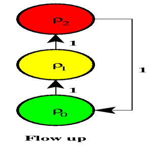
Figure 1: Flow diagram with energetic barriers. Arrows indicate the average number of variables transfered, $nT_{b,a}$, from a state $a$ to a state $b$, given that a variable in $a$ gets updated. Diagonal elements $T_{a,a}$ correspondingly are negative, accounting for the outflow. Note that variables transferring from $\rho_{1}$ to $\rho_{0}$ most first jump up in energy to $\rho_{2}$.

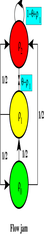
Figure 2: Same as Fig. 2, but with a model leading to a jam. Variables can only transfer from $\rho_{2}$ to $\rho_{0}$ through $\rho_{1}$, but only if $\rho_{1}<\theta$. Once $\rho_{1}=\theta$, flow down from $\rho_{2}$ ceases until $\rho_{1}$ reduces again.

To demonstrate the use of these equations, we consider a simple model of an energetic barrier with only three states $(\alpha=2)$ and a constant flow matrix $T_{b,a}=[-\delta_{b,a}+\delta_{(2+b~{}{\rm mod}~{}3),a}]/n$, depicted in Fig. 2. Here, variables in $\rho_{1}$ can only reach their lowest-energy state in $\rho_{0}$ by first jumping up in energy to $\rho_{2}$. Eq. (3) gives

$${\dot{\rho}}_{0}=\frac{1}{n}\left(-Q_{0}+Q_{2}\right),\quad{\dot{\rho}}_{1}=\frac{1}{n}\left(Q_{0}-Q_{1}\right),\quad{\dot{\rho}}_{2}=\frac{1}{n}\left(Q_{1}-Q_{2}\right),$$ (18)

with ${\bf Q}$ discussed in Sec. III.2 for the variants of EO.

Given ${\bf T}$, we can now also determine the update probabilities for Metropolis according to Eqs. (17). Note that for $a=2$ we can evaluate the $min$ as $1$, since $\sum_{b}bT_{b,a}<0$ always, while for $a=0,1$ the $min$ always evaluates to the exponential. Properly normalized, we obtain

$$Q_{0} = \frac{\rho_{0}e^{-\beta/2}}{(1-e^{-\beta/2})\rho_{2}+e^{-\beta/2}},\quad Q_{1}=\frac{\rho_{1}e^{-\beta/2}}{(1-e^{-\beta/2})\rho_{2}+e^{-\beta/2}},$$

$$\vskip 6.0pt plus 2.0pt minus 2.0ptQ_{2} = \frac{\rho_{2}}{(1-e^{-\beta/2})\rho_{2}+e^{-\beta/2}}.$$ (19)

It is now very simple to obtain the stationary solution: For ${\dot{\bf\rho}}=0$, Eqs. (18) yields $Q_{0}=Q_{1}=Q_{2}=1/3$, and we obtain from Eq. (12) for $\tau$-EO:

$$\rho_{0}=1-\left(\frac{1}{3}n^{\tau-1}+\frac{2}{3}\right)^{\frac{1}{1-\tau}},\quad\rho_{2}=\left(\frac{2}{3}n^{\tau-1}+\frac{1}{3}\right)^{\frac{1}{1-\tau}},\quad\rho_{1}=1-\rho_{0}-\rho_{2},$$ (20)

for $\mu$-EO:

$$\rho_{0}=\frac{1}{\mu}\ln\left[\frac{2}{3}+\frac{1}{3}e^{\mu\left(1-1/n\right)}\right],\quad\rho_{2}=1-\frac{1}{\mu}\ln\left[\frac{1}{3}+\frac{2}{3}e^{\mu\left(1-1/n\right)}\right],\quad\rho_{1}=1-\rho_{0}-\rho_{2},$$ (21)

and for Metropolis:

$$\rho_{0}=\frac{1}{2+e^{-\beta/2}},\quad\rho_{1}=\frac{1}{2+e^{-\beta/2}},\quad\rho_{2}=\frac{e^{-\beta/2}}{2+e^{-\beta/2}}.$$ (22)

For EO with threshold updating, we obtain

$$\rho_{0} = \frac{1}{3}-\frac{1}{3n}-\frac{s}{n}-\frac{1}{3nr}\ln\left[1+e^{r(n-s)}\right]$$

$$~{}~{}~{}~{}+\frac{1}{nr}\ln\left[\left(e^{nr}+e^{rs}\right)\left(1+e^{r(1-s)}\right)^{\frac{1}{3}}+e^{\frac{r}{3}(2n+1)}\left(1+e^{r(n-s)}\right)^{\frac{1}{3}}\right],$$

$$\vskip 6.0pt plus 2.0pt minus 2.0pt\rho_{2} = \frac{1}{3}+\frac{2}{3n}+\frac{s}{n}-\frac{2}{3nr}\ln\left[1+e^{r(n-s)}\right]$$ (23)

$$~{}~{}~{}~{}+\frac{1}{nr}\ln\left[\left(e^{nr}+e^{rs}\right)\left(1+e^{r(1-s)}\right)^{\frac{2}{3}}+e^{\frac{r}{3}(n+2)}\left(1+e^{r(n-s)}\right)^{\frac{2}{3}}\right],$$

and, assuming a threshold anywhere between $1<s<n$, for $r\to\infty$:

$$\rho_{0}=1-\frac{2s+1}{3n},\quad\rho_{2}=\frac{s+2}{3n},\quad\rho_{1}=1-\rho_{0}-\rho_{2}$$ (24)

Therefore, according to Eq. (4), Metropolis reaches its best, albeit sub-optimal, cost $\epsilon=1/4>0$ at $\beta\to\infty$, due to the energetic barrier faced by the variables in $\rho_{1}$, see Fig. 2. (Since fluctuations from the mean are suppressed in this model, even a slowly decreasing temperature schedule as in Simulated Annealing would not improve results.) In turn, $\mu$-EO does reach optimality ($\rho_{0}=1$, hence $\epsilon=0$), but only for $\mu\to\infty$. Note that in this limit, $\mu$-EO reduces back to the “basic” version of EO discussed in Sec. III.1. The result for threshold updating in EO are more promising: near-optimal results are obtained, to within $O(1/n)$, for any finite threshold $s$. But again, results are best for small $s\to 1$, in which limit we revert back to “basic” EO.

The result for $\tau$-EO is most remarkable: For $n\to\infty$ at $\tau<1$ EO remains sub-optimal, but reaches the optimal cost for all $\tau>1$! As discussed in Ref. eo_jam , this transition at $\tau=1$ separates an (ergodic) random walk phase with too much fluctuation, and a greedy descent phase with too little fluctuation, which would trap $\tau$-EO in problems with broken ergodicity Palmer . This transition derives generically from the scale-free power-law in Eq. (8), as was already argued on the basis of numerical results for real NP-hard problems in Refs. BoPe1 ; BoPe2 .

V Jamming Model for $\mu$-EO

In this section, we revisit the “jammed” model treated in Ref. eo_jam for $\tau$-EO and repeat that calculation for $\mu$-EO. As in the example in Sec. IV, $\mu$-EO proves inferior to $\tau$-EO: Lacking the phase of optimal performance in the $\tau$-parameter space, the required fine-tuning of $\mu$ does not succeed in satisfying the conflicting constraints imposed on the search.

Naturally, the range of phenomena found in a local search of NP-hard problems is not limited to energetic barriers. After all, so far we have only considered constant entries for $T_{b,a}$. Therefore, in our next model we want to consider the case of ${\bf T}$ depending linearly on the $\rho_{i}$ discussed in Ref. eo_jam for $\tau$-EO. This model highlights significant differences between the $\tau$-EO and the $\mu$-EO implementation.

From Fig. 2, we can read off ${\bf T}$ and obtain for Eq. (3):

$${\dot{\rho}}_{0} = \frac{1}{n}\left[-Q_{0}+\frac{1}{2}Q_{1}\right],$$

$$\vskip 6.0pt plus 2.0pt minus 2.0pt{\dot{\rho}}_{1} = \frac{1}{n}\left[\frac{1}{2}Q_{0}-Q_{1}+(\theta-\rho_{1})Q_{2}\right],$$ (25)

. and ${\dot{\rho}}_{2}=-{\dot{\rho}}_{0}-{\dot{\rho}}_{1}$ from Eq.(6). Aside from the dependence of ${\bf T}$ on $\rho_{1}$, we have also introduced the threshold parameter $\theta$. In fact, if $\theta\geq 1$, the model behaves effectively like the previous model, and for $\theta\leq 0$ there can be no flow from state $2$ to the lower states at all. The interesting regime is the case $0<\theta<1$, where further flow from state $2$ into state $1$ can be blocked for increasing $\rho_{1}$, providing a negative feed-back to the system. In effect, the model is capable of exhibiting a “jam” as observed in many models of glassy dynamics Jaeger ; Ben-Naim ; Ritort , and which is certainly an aspect of local search processes. Indeed, the emergence of such a “jam” is characteristic of the low-temperature properties of spin glasses and real optimization problems: After many update steps most variables freeze into a near-perfect local arrangement and resist further change, while a finite fraction remains frustrated (temporarily in this model, permanently in real problems) in a poor local arrangement PSAA . More and more of the frozen variables have to be dislodged collectively to accommodate the frustrated variables before the system as a whole can improve its state. In this highly correlated state, frozen variables block the progression of frustrated variables, and a jam emerges.

Inserting the set of Eqs. (14) for $\alpha=2$ into the model in Eqs. (25), we obtain

$${\dot{\rho}}_{0} = \frac{1}{n}\frac{1}{e^{\mu\left(1-1/n\right)}-1}\left[1-\frac{3}{2}e^{\mu\rho_{0}}+\frac{1}{2}e^{\mu\left(\rho_{0}+\rho_{1}\right)}\right],$$

$$\vskip 6.0pt plus 2.0pt minus 2.0pt{\dot{\rho}}_{1} = \frac{1}{n}\frac{1}{e^{\mu\left(1-1/n\right)}-1}\left[-\frac{1}{2}+\frac{3}{2}e^{\mu\rho_{0}}-e^{\mu\left(\rho_{0}+\rho_{1}\right)}+(\theta-\rho_{1})\left(e^{\mu\left(1-1/n\right)}-e^{\mu\left(\rho_{0}+\rho_{1}\right)}\right)\right],$$ (26)

At large times $t$, the steady state solution, ${\dot{\bf\rho}}=0$, yields for $\rho_{0}$ after eliminating $\rho_{1}$ the implicit equation

$$0=\frac{3}{2}-\frac{3}{2}e^{\mu\rho_{0}}+\left[\theta-\frac{1}{\mu}\ln\left(3-2e^{-\mu\rho_{0}}\right)\right]\left(e^{\mu\left(1-1/n\right)}-3e^{\mu\rho_{0}}\right),$$ (27)

and according to Eq. (4), again eliminating $\rho_{1}$ and $\rho_{2}$ in favor of $\rho_{0}$, we can express the cost per variable as

$$\epsilon = 1-\rho_{0}-\frac{1}{2\mu}\ln\left(3-2e^{-\mu\rho_{0}}\right),$$ (28)

$$\sim \frac{1}{\mu}\ln\left[\sqrt{3}\left(1+\frac{1}{2\theta}\right)\right]\quad(\mu\gg 1),$$

Unlike the corresponding equations in Ref. eo_jam , which had a phase transition similar to the solution for $\tau$-EO in Sec. IV, Eqs. (27-28) have no distinct features. In fact, as shown in Fig. 3, $\epsilon(\mu)$ behaves similar to the solution for $\mu$-EO in Sec. IV: The relation is independent of $n$ to leading order and only for $\mu\to\infty$, $\rho_{0}\to 1$ and $\epsilon\to 0$.

While the steady state ($t\to\infty$) features of this model do not seem to be much different from the model in Sec. IV, the dynamics at intermediate times $t$ is more subtle. In particular, as was shown in Ref. eo_jam , a “jam” in the flow of variables towards better fitness may ensue under certain circumstances. The emergence of the jam depends on initial conditions, and its duration will prove to get longer for larger values of $\mu$. If the initial conditions place a fraction $\rho_{0}>1-\theta$ already into the lowest state, most likely no jam will emerge, since $\rho_{1}(t)<\theta$ for all times, and the ground state is reached in $t=O(n)$ steps. But if initially $\rho_{1}+\rho_{2}=1-\rho_{0}>\theta$, and $\mu$ is sufficiently large, $\mu$-EO will drive the system to a situation where $\rho_{1}\approx\theta$ by preferentially transferring variables from $\rho_{2}$ to $\rho_{1}$. Then, further evolution becomes extremely slow, delayed by the $\mu$-dependent, small probability that a variable in state $1$ is updated ahead of all variables in state $2$.

Clearly, this jam is not a steady state solution of Eq. (26). It is not even a meta-stable solution since there are no energetic barriers. For instance, simulated annealing at zero temperature would easily find the solution in $t=O(n)$ without experiencing a jam. In reality, a hard problem would most certainly contain combinations of jams, barriers, and possibly other features.

To analyze the jam, we consider initial conditions leading to a jam, $\rho_{1}(0)+\rho_{2}(0)>\theta$ and make the Ansatz

$$\rho_{1}(t)=\theta-\eta(t)$$ (29)

with $\eta\ll 1$ for $t\lesssim t_{\rm jam}$, where $t_{\rm jam}$ is the time at which $\rho_{0}\to 1$. To determine $t_{\rm jam}$, we apply Eq. (29) to the evolution equations in (26) to get

$${\dot{\rho}}_{0}\sim\frac{1}{n}\frac{1}{e^{\mu\left(1-1/n\right)}-1}\left[1-\frac{3}{2}e^{\mu\rho_{0}}+\frac{1}{2}e^{\mu\left(\rho_{0}+\theta\right)}\right],$$ (30)

where the relation for ${\dot{\rho}}_{1}$ merely yields a self-consistent equation to determine sub-leading corrections.

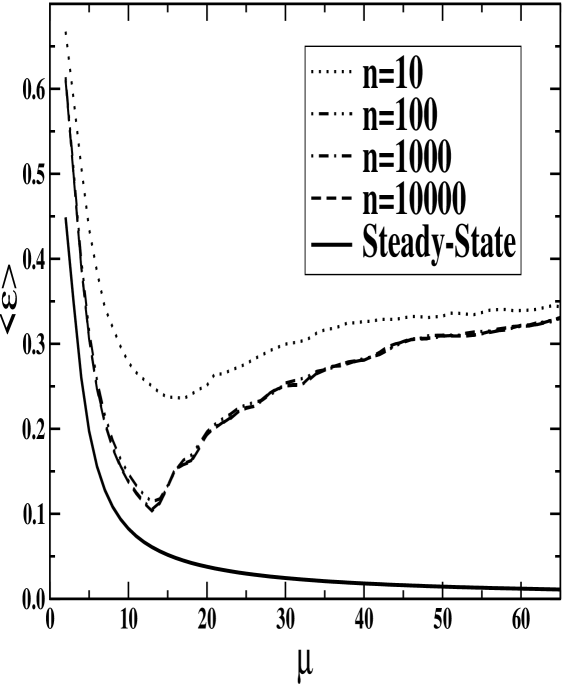
Figure 3: Plot of the energy $\langle\epsilon\rangle$ averaged over many $\mu$-EO runs after $t_{\rm max}=100n$ updates with different initial conditions as a function of $\mu$ for $n=10$, 100, 1000, and 10000 and $\theta=1/2$. Plotted also is $\epsilon=\sum_{a}a\rho_{a}/2$ as a function of $\mu$ resulting from the jam-free steady-state solution ($t\to\infty$) of Eqs. (27-28) $n=\infty$. The plots show little variability with system size for large $n$, and remain quite sub-optimal for finite $\mu$. As for $\tau\to\infty$ in Ref. eo_jam , $\langle\epsilon\rangle\to 2/3-\theta/2-\theta^{3}/6=19/48\approx 0.396$ rem1 for $\mu\to\infty$.

We can now integrate Eq. (30) from $t=0$ (assuming that any jam emerges almost instantly) up to $t_{\rm jam}$, where $\rho_{0}=1$:

$$t_{\rm jam}\sim n\left(e^{\mu}-1\right)\int_{\rho_{0}(0)}^{\rho_{0}(t_{\rm jam})=1}\frac{d\xi}{1-\left(\frac{3}{2}-\frac{1}{2}e^{\mu\theta}\right)e^{\mu\xi}}$$ (31)

The integral is easily evaluated, and we find for large values of $\mu$:

$$t_{\rm jam}\sim\frac{2n}{\mu}e^{\mu(1-\theta-\rho_{0}(0))}\quad(\mu\gg 1).$$ (32)

Instead of repeating the lengthy calculation in Ref. eo_jam for the ground state energy averaged over all possible initial conditions for finite runtime $t_{\rm max}\propto n$, we can content ourselves here with a few obvious remarks: A finite fraction of the initial conditions will lead to a jam, hence will require a runtime $t_{\rm max}\gg t_{\rm jam}$ to reach optimality. Yet, to reach a quality minimum, say, $\epsilon\sim 1/n$, would require $\mu\sim n\gg 1$ according to Eq. (28). Thus, the require runtime to resolve the jam would grow exponentially with system size $n$, since from Eq. (32) $t_{\rm jam}\sim e^{cn}$ with $c=1-\theta-\rho_{0}(0)>0$, by definition of the jam above.

In conclusion, $\mu$-EO can never quite resolve the conflicting demands of pursuing quality ground states with a strong bias for selecting variables of low fitness (i. e. $\mu\gg 1$) and the ensuing lack of fluctuations required to break out of a jam, which drives up $t_{\rm jam}$. Simulations of this model with $\mu$-EO in Fig. 3 indeed show that the best results for $\langle\epsilon\rangle$ are obtained at intermediate values of $\mu$, which converge to a large, constant error for increasing $n$. In contrast, $\tau$-EO provides a range near $\tau_{\rm opt}-1\sim 1/\ln(n)$ eo_jam with small enough $\tau$ to fluctuate out of any jam in a time near-linear in $n$ while still attaining optimal results as it does for any $\tau>1$, see e. g. Sec. IV.

VI Conclusion

We have presented a simple model to analyze the properties of local search heuristics. The model with a simple energetic barrier demonstrates the characteristics of a number of these heuristics, whether athermal (EO and its variants) or thermal (Metropolis) Boettcher05b . In particular, it plausibly describes a number of real phenomena previously observed for $\tau$-EO in a tractable way. Finally, in a more substantive comparison on a model with jamming, the exponential distribution over fitnesses, $\mu$-EO proves unable to overcome the conflicting constraints of resolving the jam while finding good solutions. This is in stark contrast with the identical calculation in Ref. eo_jam using a scale-free approach with a power-law distribution over fitnesses in $\tau$-EO. In this approach, a sharp phase transition emerges generically between an expansive but unrefined exploration on one side (“ergodic” phase), and a greedy but easily trapped search on the other (“non-ergodic” phase), with optimal performance near the transition.

References

- (1) M. R. Garey and D. S. Johnson, Computers and Intractability, A Guide to the Theory of NP-Completeness (W. H. Freeman, New York, 1979).
- (2) New Optimization Algorithms in Physics, Eds. H. Rieger and A. K. Hartmann, (Springer, Berlin, 2004).
- (3) K. F. Pal, Physica A 223, 283-292 (1996), and 233, 60-66 (1996).
- (4) A. K. Hartmann, Phys. Rev. B 59, 3617-3623 (1999), and Phys. Rev. E 60, 5135-5138 (1999).
- (5) M. Palassini and A. P. Young, Phys. Rev. Lett. 85, 3017 (2000).
- (6) J. Houdayer and O. C. Martin, Phys. Rev. Lett. 83, 1030 (1999).
- (7) S. Boettcher and A. G. Percus, Phys. Rev. Lett. 86, 5211-5214 (2001).
- (8) K. K. Bhattacharya and J. P. Sethna, Phys. Rev. E 57, 2553 (1998).
- (9) E. Tuzel and A. Erzan, Phys. Rev. E 61, R1040 (2000).
- (10) H. Frauenkron, U. Bastolla, E. Gerstner, P. Grassberger, and W. Nadler, Phys. Rev. Lett. 80, 3149-3152 (1998).
- (11) T. Prellberg and J. Krawczyk, Phys. Rev. Lett. 92, 120602 (2004).
- (12) R. G. Palmer and J. Adler, Int. J. Mod. Phys. C 10, 667 (1999).
- (13) C. Desimone, M. Diehl, M. Jünger, P. Mutzel, G. Reinelt, G. Rinaldi, J. Stat. Phys. 80, 487-496 (1995).
- (14) Modern Heuristic Search Methods, Eds. V. J. Rayward-Smith, I. H. Osman, and C. R. Reeves (Wiley, New York, 1996).
- (15) S. Kirkpatrick, C. D. Gelatt, and M. P. Vecchi, Science 220, 671-680 (1983).
- (16) P. Salamon, P. Sibani, and R. Frost, Facts, Conjectures, and Improvements for Simulated Annealing (Society for Industrial & Applied Mathematics, 2002).
- (17) J. Holland, Adaptation in Natural and Artificial Systems (University of Michigan Press, Ann Arbor, 1975).
- (18) S. Boettcher and A. G. Percus, Artificial Intelligence 119, 275-286 (2000).
- (19) S. Boettcher and A. G. Percus, in GECCO-99: Proceedings of the Genetic and Evolutionary Computation Conference (Morgan Kaufmann, San Francisco, 1999), 825-832.
- (20) S. Boettcher and A. G. Percus, Physical Review E 64, 026114 (2001).
- (21) S. Boettcher and A. G. Percus, Phys. Rev. E 69, 066703 (2004).
- (22) S. Boettcher, Phys. Rev. B 67, R060403 (2003).
- (23) S. Boettcher, Extremal Optimization for Sherrington-Kirkpatrick Spin Glasses, Euro. Phys. J. B (in press), condmat/0407130.
- (24) S. Boettcher, J. Math. Phys. A 32, 5201-5211 (1999).
- (25) N. Metropolis, A.W. Rosenbluth, M.N. Rosenbluth, A.H. Teller and E. Teller, Equation of state calculations by fast computing machines, J. Chem. Phys. 21 (1953) 1087–1092.
- (26) J. Dall and P. Sibani Comp. Phys. Comm. 141, 260-267 (2001).
- (27) S. Boettcher and P. Sibani, Euro. Phys. J. B 44, 317-326 (2005).
- (28) S. Meshoul and M. Batouche, Lecture Notes in Computer Science 2449, 330-337 (2002).
- (29) S. Meshoul and M. Batouche, Int. J. Pattern Rec. and AI 17, 1111-1126 (2003).
- (30) E. Yom-Tov, A. Grossman, and G. F. Inbar, Biological Cybernatics 85, 395-399 (2001).
- (31) F. L. Sousa, V. Vlassov and F. M. Ramos, Heat Transf. Eng. 25, 34-45 (2004).
- (32) T. Zhou, W.-J. Bai, L.-J. Cheng, and B.-B. Wang, Phys. Rev. E 72, 016702 (2005).
- (33) M. E. Menai and M. Batouche, Lecture Notes in Computer Science 2718, 592-603 (2003).
- (34) M. E. Menai and M. Batouche, in Proceedings of the International Conference on Artificial Intelligence, IC-AI2003, Eds. H. R. Arabnia et. al., 257-262 (2003).
- (35) J. Duch and A. Arenas, Community detection in complex networks using Extremal Optimization, cond-mat/0501368.
- (36) J.-S. Wang and Y. Okabe, J. Phys. Soc. Jpn. 72, 1380 (2003).
- (37) R. N. Onody and P. A. de Castro, Physica A 322, 247-255 (2003).
- (38) S. Boettcher and M. Grigni, J. Phys. A. 35, 1109 (2002).
- (39) A. A. Middleton, Phys. Rev. E 69, 055701 (R) (2004).
- (40) F. L. de Sousa and V. Vlassov and F. M. Ramos, Lecture Notes in Computer Science 2723, 375-376 (2003).
- (41) F. L. de Sousa, F. M. Ramos, R. L. Galski, and I. Muraoka, in Recent Developments in Biologically Inspired Computing, Eds. L. N. De Castro and F. J. Von Zuben (Idea Group Inc., 2004).
- (42) F. Heilmann, K.-H. Hoffmann, and P. Salamon, Europhys. Lett. 66, 305-310 (2004).
- (43) K.-H. Hoffmann, F. Heilmann, and P. Salamon, Phys. Rev. E 70, 046704 (2004).
- (44) Landscape Paradigms in Physics and Biology, Ed. H. Frauenfelder (Elsevier, Amsterdam, 1997).
- (45) M. Mézard, G. Parisi, and M. A. Virasoro, Spin Glass Theory and Beyond, (World Scientific, Singapore, 1987).
- (46) F. T. Bantilan and R. G. Palmer, J. Phys. F: Metal Phys. 11, 261-266 (1981).
- (47) H. M. Jaeger, S. R. Nagel, R. P. Behringer, Rev. Mod. Phys 68 1259-1273 (1996).
- (48) E. Ben-Naim, J. B. Knight, E. R. Nowak, H. M. Jaeger, and S. R. Nagel, Physica D 123, 380-385 (1998).
- (49) F. Ritort, Phys. Rev. Lett. 75, 1190-1193 (1995).
- (50) R. G. Palmer, D. L. Stein, E. Abrahams, and P. W. Anderson, Phys. Rev. Lett. 53, 958 (1984).
- (51) Ref. eo_jam has in error in Eq. (28): The general expression for the energy in the integrand, , should be replaced by in the jam, which leads to this value for for large or , instead of quoted there.