Propagation of Light in Photonic Crystal Fibre Devices

Abstract

We describe a semi-analytical approach for three-dimensional analysis of photonic crystal fibre devices. The approach relies on modal transmission-line theory. We offer two examples illustrating the utilization of this approach in photonic crystal fibres: the verification of the coupling action in a photonic crystal fibre coupler and the modal reflectivity in a photonic crystal fibre distributed Bragg reflector.

1 Introduction

Photonic crystal fibres (PCFs), whose cladding is composed of a two-dimensional (2D) photonic crystal [1, 2], may confine and guide light through either a photonic bandgap effect [3, 4] or by an effective high refractive index guiding mechanism [5, 6]. Both classes of fibres have been the subject of numerous research and for a review we refer to Refs. [7, 8] and references therein. The latter class of PCFs has attractive features such as, broad-band single-mode (SM) operation [9], possibilities for dispersion engineering [10, 11], and tailorable mode area [12]. The 2D photonic crystal of the cladding not only provides more design freedom on engineering basic properties of the fibre, but also broadens the potential application of PCFs by the freedom to remove more air holes from the cladding [13, 14, 15] or by introducing additional materials to the air holes [16, 17, 18, 19, 20], both of which facilitate novel device operations based on PCFs. In the present work, the ”PCF device” term is restricted to the ones obtained by removing some holes from the cladding such as, PCF couplers [13, 14], PCF polarization beam splitters [15], or PCF distributed Bragg reflectors [21].

In the present paper, we describe an approach, which relies on modal transmission-line theory (MTLT), for three-dimensional (3D) investigations of the propagation of an optical beam launched into a PCF device. According to our knowledge only the finite element beam propagation method (FE-BPM) [22] has been adopted and utilized for doing such simulations. The FE-BPM is numerically robust, versatile, and applicable to a wide variety of structures. Unfortunately, this is often achieved at the expense of long computational times and large memory requirements, both of which can become critical issues especially when structures with large dimensions are considered or when used within an iterative design environment.
MTLT, which has been developed for modelling multi-layered periodic media [23, 24, 25, 26, 27], has been used for analysis of distributed feedback (DFB) lasers [25, 26], quantum well infrared photodetectors (QWIP) [28], holographic power splitter/combiners [29] and grating assisted integrated optics devices [30]. Recently, it has also successfully been applied in a study of radiation fields from end-facet PCFs [31]. MTLT relies on a plane-wave expansion of electromagnetic fields in the periodic media. Interpreting the plane waves as transmission-lines provides a systematic framework for study of wave propagation in multi-layered periodic media. Besides that, one can exploit all the concepts and methods of transmission-line theory [32] and electrical network theory [33] for the study of wave propagation. MTLT has recently been developed for modal analysis of arbitrary shape optical waveguides [34]. Here, we add a novel approach to this theory and utilize it for a three-dimensional study of propagation of light in photonic crystal fibre devices.

The remaining part of the paper is organized as follows. In Section 2, we give a brief account of MTLT and describe the approach we use. In Section 3 we investigate examples that illustrate the utilization of this approach in the modelling of PCF devices. Finally, conclusions are given in Section 4.

2 Formalism

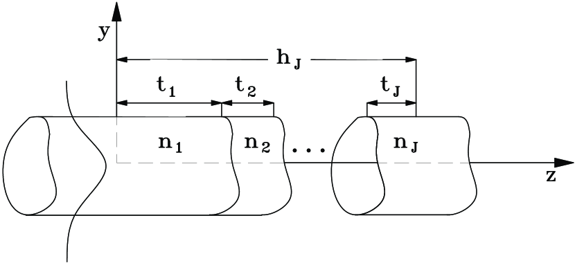
Figure 1: General case of a three-dimensional multi-layered structure.

The typical PCF device that we have in mind is composed of $J$ layers with different relative permittivity functions $\epsilon_{rj}(x,y),~{}j=1,2,\cdots,J$, which is illustrated in figure 1. We define $z_{j}$ as a convenient local coordinate obeying $0\leq z_{j}=z-h_{j-1}\leq t_{j}$ and we consider wave propagation along the longitudinal direction of the structure, i.e. $z$-axis. Throughout this paper we consider non-magnetic materials with relative permeability $\mu_{r}=1$ and all electromagnetic fields have a harmonic temporal dependence, $\exp(i\omega t)$. PCF devices with the typical shape shown in figure 1, usually confine light within the fibre core or cores. However, some application such as long-period fibre Bragg gratings do not share this feature so in the present study we exclude these applications. For the applications with spatially localized modes we use a super-cell approach and repeat the structure in the transverse $xy$-plane, along $x$ and $y$ directions with periodicities of $T_{x}$ and $T_{y}$, respectively. It is assumed that the periodically repeated devices are separated by a sufficient amount of background region, here microstructured cladding, that their electromagnetic fields do not affect each other significantly.

We want to study a PCF device when it is illuminated with an incident field ${\vec{E}}_{inc}({\vec{r}})$ propagating in layer 1 of the structure shown in figure 1. This incident field is a solution to the source-free Maxwell equations in the PCF with the refractive index profile of layer 1. In this section we briefly address MTLT and modal analysis of optical waveguides using this theory. Subsequently we describe an approach, based on MTLT, for investigating the scattering and propagation of light in PCF devices. Throughout the paper, vectorial components are denoted by an arrow placed above them. The bold-style notation with uppercase and lowercase characters is used to designate matrices and vectors, respectively.

2.1 Modal Transmission-Line Theory

Embody a periodic medium with permittivity variation $\epsilon_{0}\epsilon_{r}(x,y)=\epsilon_{0}\epsilon_{r}(x+T_{x},y+T_{y})$ and permeability $\mu_{0}$. The permittivity can then conveniently be expressed in the form of a two-dimensional Fourier series [26]

$$\epsilon_{r}(x,y)=\lim_{M,N\longrightarrow\infty}\sum_{m=-M}^{M}\sum_{n=-N}^{N}{\tilde{\epsilon}}_{mn}\exp\Big{(}{-im\frac{2\pi}{T_{x}}x}\Big{)}\exp\Big{(}{-in\frac{2\pi}{T_{y}}y}\Big{)}$$ (1)

where

$${\tilde{\epsilon}}_{mn}=\frac{\displaystyle{1}}{\displaystyle{T_{x}T_{y}}}\int_{0}^{T_{x}}\int_{0}^{T_{y}}\epsilon_{r}(x,y)\exp\Big{(}{im\frac{2\pi}{T_{x}}x}\Big{)}\exp\Big{(}{in\frac{2\pi}{T_{y}}y}\Big{)}dydx~{}.$$ (2)

The electromagnetic fields must of course reflect the periodicity of $\epsilon_{r}(x,y)$ and according to the Floquet–Bloch theorem the fields in the doubly periodic medium are pseudo-periodic functions [26]

$${{{\vec{A}}}({\vec{r}})=\lim_{M,N\longrightarrow\infty}\sum_{m=-M}^{M}\sum_{n=-N}^{N}{{\vec{a}}_{mn}(z)}}\exp\Big{[}{-i\Big{(}K_{x0}+m\frac{2\pi}{T_{x}}}\Big{)}x\Big{]}\exp\Big{[}{-i\Big{(}K_{y0}+n\frac{2\pi}{T_{y}}}\Big{)}y\Big{]}$$ (3)

where, ${\vec{K}_{0}}=K_{x0}\hat{x}+K_{y0}\hat{y}$ is the Bloch wave-vector and ${\vec{A}}$ can be any of the electromagnetic fields ${\vec{E}},~{}{\vec{H}}$, or ${\vec{D}}$. In order to facilitate calculations in matrix form, we introduce ${\bf\vec{e}},~{}{\bf\vec{h}}$, and ${\bf\vec{d}}$ vectors whose elements are ${\vec{e}}_{mn},~{}{\vec{h}}_{mn}$, and ${\vec{d}}_{mn}$, respectively. The dimension of each vectorial component of the ${\bf\vec{e}},~{}{\bf\vec{h}}$, or ${\bf\vec{d}}$ vectors in Cartesian coordinates (i.e. ${\bf e_{x}}$, ${\bf e_{y}}$, ${\bf e_{z}}$, ${\bf h_{x}}$, etc.) is $1\times(2N+1)(2M+1)$. Using these vectors, the constitutive relation ${\vec{D}}=\epsilon_{0}\epsilon_{r}{\vec{E}}$ converts into ${\bf\vec{d}}=\epsilon_{0}{\bf N}{\bf\vec{e}}$, where ${\bf N}$ is a square matrix whose elements are $\tilde{\epsilon}_{mn}$ and they are arranged in ${\bf N}$ in such a way that the equality ${\bf\vec{d}}=\epsilon_{0}{\bf N}{\bf\vec{e}}$ holds.
The temporal harmonic electromagnetic fields in a dielectric medium are solutions of the following source-free Maxwell equations

$$\left\{\begin{array}[]{r r r}\nabla\times{\vec{E}}({\vec{r}})&=&-i\omega\mu_{0}{\vec{H}}({\vec{r}})\\ \nabla\times{\vec{H}}({\vec{r}})&=&i\omega{\vec{D}}({\vec{r}})\end{array}\right.$$ (6)

Using (1), (3), and vectors ${\bf\vec{e}},~{}{\bf\vec{h}}$ and ${\bf\vec{d}}$ in the source-free Maxwell equations (6), these equations are transformed into the following system of differential equations:

$$\left\{\begin{array}[]{r r r}\frac{\displaystyle{d{\bf v}}}{\displaystyle{dz}}&=&-i\omega{\bf L}{\bf i}\\ \\ \frac{\displaystyle{d{\bf i}}}{\displaystyle{dz}}&=&-i\omega{\bf C}{\bf v}\end{array}\right.$$ (10)

or

$$\left\{\begin{array}[]{r r r}\frac{\displaystyle{d^{2}{\bf v}}}{\displaystyle{dz^{2}}}&=&-\omega^{2}{\bf L}{\bf C}{\bf v}\\ \\ \frac{\displaystyle{d^{2}{\bf i}}}{\displaystyle{dz^{2}}}&=&-\omega^{2}{\bf C}{\bf L}{\bf i}\end{array}\right.$$ (14)

where ${\bf L}$ and ${\bf C}$ are obtained in the calculations [26] and

$${\bf v}=\left[\begin{array}[]{c}{\bf e_{y}}\\ {\bf e_{x}}\end{array}\right],~{}{\bf i}=\left[\begin{array}[]{c}{\bf h_{x}}\\ -{\bf h_{y}}\end{array}\right]~{}.$$ (15)

Equation (10) has the well-known form of telegraphist’s equations for a multi-conductor transmission-line [32] and we have emphasized the analogy by the choice of symbols so that e.g. ${\bf i}$ and ${\bf v}$ are interpreted as effective currents and voltages, respectively. Likewise, inductance and capacitance matrices of the multi-conductor transmission-line are denoted by ${\bf L}$ and ${\bf C}$, respectively. In equation (14), $\omega^{2}{\bf LC}$ and $\omega^{2}{\bf CL}$ are matrices with non-zero off-diagonal elements. We can formally diagonalize $\omega^{2}{\bf LC}$ and $\omega^{2}{\bf CL}$ matrices using relations $\omega^{2}{\bf LC}={\bf PK^{2}P^{-1}}$ and $\omega^{2}{\bf CL}={\bf QK^{2}Q^{-1}}$, where ${\bf K^{2}}$ is a diagonal matrix. The diagonal elements of ${\bf K^{2}}$ are eigenvalues of $\omega^{2}{\bf LC}$ or $\omega^{2}{\bf CL}$. Here, ${\bf P}$ and ${\bf Q}$ are matrices whose columns are the eigenvectors of their relevant non-diagonal matrices. Once the ${\bf K^{2}}$ and ${\bf P}$ have been determined, the matrix ${\bf Q}$ is also given by $\omega{\bf CPK^{-1}}$.
From the above discussion it follows that (14) may be transformed into

$$\left\{\begin{array}[]{r r r}\frac{\displaystyle{d^{2}{\bf\widehat{v}}}}{\displaystyle{dz^{2}}}&=&-{\bf K^{2}\widehat{v}}\\ \\ \frac{\displaystyle{d^{2}{\bf\widehat{i}}}}{\displaystyle{dz^{2}}}&=&-{\bf K^{2}\widehat{i}}\end{array}\right.$$ (19)

where

$${\bf{v}}={\bf P}{\bf\widehat{v}}~{}~{},~{}~{}{\bf i}={\bf Q\widehat{i}}.$$ (20)

In this new basis the transmission-lines are uncoupled and one may, in analogy with conductance eigen-channels in quantum transport [35], think of these new lines as the eigen-lines of the transmission-line system. Wave propagation in the periodic medium is described by ${\bf K^{2}}$, ${\bf P}$, ${\bf Q}$, see (19) and (20).
Evidently from MTLT, the $\omega^{2}{\bf LC}$ describes the propagation characteristics of longitudinal space harmonics. Eigenvalues of this matrix specify the square values of propagation constants of space harmonics. The propagation constants are obtained from the diagonal matrix ${\bf K^{2}}$ considering the following condition [24]:

$$\textrm{Im}(K_{k})+\textrm{Re}(K_{k})<0.$$ (21)

Electromagnetic fields of each space harmonic with a specified propagation constant are determined from its relevant eigenvector.

2.2 Equivalent Network of Multi-Layered Media

Consider the typical structure shown in figure 1. The modelling task begins by periodically repeating the device in the transverse $xy$-plane with sufficiently large periodicities. As discussed above, wave propagation in each layer of this periodically repeated structure could be modelled by a transmission-line network whose behavior is described by (19). Schematically, the equivalent transmission-line network of the j-th layer of this structure is depicted in figure 2 (a). In this figure the box containing $P_{j},~{}Q_{j}$ represents the consideration in (20).
A concise and effective formulation of voltages and currents of this transmission-line network can be described by:

$$\left\{\begin{array}[]{r r r}{\bf\widehat{{v}}_{j}}&=&{\bf\exp}[-i{\bf K_{j}}(z_{j}-t_{j})]{\bf{\widehat{v}}_{j,inc}}+{\bf\exp}[i{\bf K_{j}}(z_{j}-t_{j})]{\bf{\widehat{v}}_{j,r}}\\ \\ {\bf\widehat{{i}}_{j}}&=&{\bf\exp}[-i{\bf K_{j}}(z_{j}-t_{j})]{\bf{\widehat{i}}_{j,inc}}-{\bf\exp}[i{\bf K_{j}}(z_{j}-t_{j})]{\bf{\widehat{i}}_{j,r}}\end{array}\right.$$ (25)

where ${\bf{\widehat{v}}_{j,inc}},~{}{\bf{\widehat{i}}_{j,inc}},~{}{\bf{\widehat{v}}_{j,r}}$, and ${\bf{\widehat{i}}_{j,r}}$ are vectors for the incident voltage, incident current, reflected voltage, and reflected current, respectively. The ${\bf K_{j}}=\textrm{diag}(K_{j1},K_{j2},\cdots,K_{jk},\cdots)$ is a diagonal matrix obtained by computing the square root of the ${\bf K_{j}^{2}}$ matrix. The ${\bf\exp}[-i{\bf K_{j}}(t_{j}-z_{j})]$ is also a diagonal matrix with diagonal elements ${\exp[-K_{jk}(t_{j}-z_{j})]}$.
Essential electromagnetic boundary conditions could be simply satisfied at the interface of two different layers by the continuity of voltages and currents in transmission-line theory. At the interface of typical different $l$ and $l+1$ layers, illustrated in figure 2 (b), the continuity rule is described by:

$$\left\{\begin{array}[]{r r r}{\bf P_{j}{\widehat{v}}_{tj}}&=&{\bf P_{j+1}{\widehat{v}}_{0,j+1}}\\ {\bf Q_{j}{\widehat{i}}_{tj}}&=&{\bf Q_{j+1}{\widehat{i}}_{0,j+1}}\end{array}\right.$$ (28)

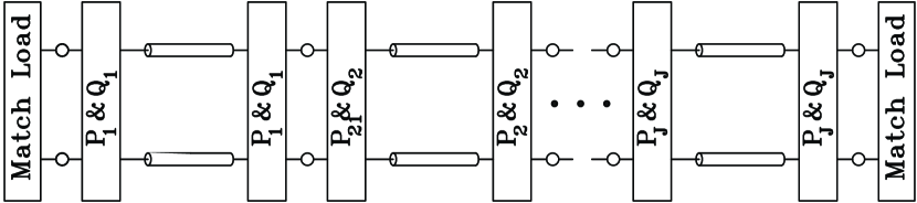
Figure 3: Equivalent transmission-line network of the multi-layered structure shown in Fig. 1.

where ${\bf{\widehat{v}}_{tj}}$, ${\bf{\widehat{v}}_{0,j+1}}$, ${\bf{\widehat{v}}_{tj}}$, and ${\bf{\widehat{v}}_{0,j+1}}$ have been defined in figure 2. On the basis of MTLT the transmission-line network of the periodically repeated typical PCF device is illustrated in figure 3. In the equivalent network of figure 3 and also in numerical simulation a total height of $h_{J}$ is considered. At the beginning ($z=0$) and the end ($z=h_{J}$) of the structure, the well-known radiation condition of electromagnetic theory is applied, which is depicted in the equivalent network by match load. Here we exploit a primary feature of radiation condition; i.e. the zero reflection at these points.

2.3 The Approach

Consider the structure shown in figure 1. When this structure is illuminated with an incident electromagnetic field ${\vec{E}}_{inc}({\vec{r}})$, propagating in layer 1 along the positive direction of $z$-axis, the total field in layer 1, ${\vec{E}}_{1}({\vec{r}})$, is given by

$${\vec{E}}_{1}({\vec{r}})={\vec{E}}_{inc}({\vec{r}})+{\vec{E}}_{1,r}({\vec{r}})$$ (29)

where ${\vec{E}}_{1,r}({\vec{r}})$ is the reflected field inside layer 1. The incident field is usually a fibre mode so for investigating its interaction with other layers we must calculate it and then calculate ${\vec{E}}_{1,r}({\vec{r}})$ and finally ${\vec{E}}_{1}({\vec{r}})$. From the known field at layer 1, we calculate the fields in other layers utilizing equations (25) and (28).
Since the incident field ${\vec{E}}_{inc}({\vec{r}})$ is a guided mode of the waveguide with refractive index profile of layer 1, we could determine it utilizing MTLT, exploiting the features of transmission-lines [34]. This calculation is achieved by examining the out of plane propagation of a periodic medium whose refractive index variation is obtained by periodically repeating the waveguide in transverse plane with sufficiently large periodicities. Evidently from transmission-line theory, the matrix $\omega^{2}{\bf LC}$ contains the information of the out of plane propagating waves, called space harmonics in the field of diffraction grating [23]. Eigenvalues of the matrix $\omega^{2}{\bf LC}$, diagonal elements of ${\bf K^{2}}$, specify squared-values of propagation constants of these space harmonics. Each column of the matrix ${\bf P}$, an eigenvector of the matrix $\omega^{2}{\bf LC}$, describe the electric field profile of its relevant eigenvalue. Among the space harmonics the ones whose field profiles are localized within the waveguide specify guided modes of the waveguide. In index guiding waveguides this condition is simplified to the refractive index guiding condition.
Through the modal analysis of the fibre with layer 1 refractive index profile we determine ${\bf{\widehat{v}}_{j,inc}}(z=0)$. Afterwards, for complete determination of field in the first layer, calculation of ${\bf{\widehat{v}}_{j,r}}(z=0)$ and ${\bf{\widehat{i}}_{j,r}}(z=0)$ is also required. These values are obtained by the following relations:

$$\left\{\begin{array}[]{r r r}{\bf{\widehat{v}}_{j,r}}(z=0)&=&{\bf R^{u}_{01}}{\bf{\widehat{v}}_{j,inc}}(z=0)\\ {\bf{\widehat{i}}_{j,r}}(z=0)&=&{\bf R^{u}_{01}}{\bf{\widehat{i}}_{j,inc}}(z=0)\end{array}\right.$$ (32)

where ${\bf R^{u}_{01}}$ is the upward reflectance matrix at $z=0$. Generally we define ${\bf R^{u}_{zj}}$ as the reflectance matrix of a propagating wave along the positive direction of z-axis at the local geometry $z_{j}$; for instance ${\bf R^{u}_{01}}$ is the upward reflectance matrix at $z_{j}=0$ for $j=1$. The variation of ${\bf R^{u}_{zj}}$ along $z$ is treated by the following relation [37]

$$\left\{\begin{array}[]{r r r}{\bf R_{tj}}&=&F_{rj}({\bf R_{0,j+1}})\\ {\bf R_{oj}}&=&\exp({\bf K_{j}}x){\bf R_{tj}}\exp({\bf K_{j}}x)\end{array}\right.$$ (35)

where $F_{rj}({\bf R_{0,j+1}})$ is composed of the following set of equations:

$$\left\{\begin{array}[]{r r r}{\bf R_{tj}}&=&({\bf Z_{tj}-I})({\bf Z_{tj}+I})^{-1}\\ {\bf Z_{tj}}&=&{\bf P_{j}^{-1}P_{j+1}Z_{0,j+1}Q^{-1}_{j+1}Q_{j}}\\ {\bf Z_{0,j+1}}&=&{\bf(I+R_{0,j+1})(I-R_{0,j+1})^{-1}}\end{array}\right.$$ (39)

Computation of ${\bf R^{u}_{01}}$ is started from the topmost layer, where the reflectance is zero. Considering (35) and (39) at each layer and interface of layers, the ${\bf R^{u}_{01}}$ would be calculated. From the known ${\bf R^{u}_{01}}$, the ${\bf{\widehat{v}_{1,r}}}$ and ${\bf{\widehat{i}_{1,r}}}$ are determined by Equation (32). Electromagnetic fields at other points of the first layer would be computed using (29). Inside other layers, electromagnetic fields will be calculated using (25) and (28).

3 Validation and Numerical Implementations

In this section, several examples will be considered to illustrate and also validate the utilization of the proposed approach.

3.1 PCF coupler

The cross-section of the PCF-coupler we want to study is depicted in the inset of figure 4. It is composed of a triangular lattice of air-holes in silica with two missing air holes. We validate the described approach in the present paper by verifying the coupling action of the coupler and comparing the obtained coupling length through this approach with the one obtained by considering even and odd modes. In the simulation the pitch, $\Lambda=7.2\,{\rm\mu m}$, and normalized hole-diameter to the pitch, $d/\Lambda=0.45$ have been set. We perform the simulation at the normalized wavelength $\lambda/\Lambda=2\pi c/(\omega\Lambda)=0.1$.
In simulation it is assumed that the light is launched into one core of the coupler, for instance core A, by butt-coupling of a similar single-core fibre whose core is aligned to the core A. The coupler and the fibre coupled to it constitute a two layer medium, which could be considered an example of the general case of figure 1.

As it is described in Section 2.2, at first we repeat the structure periodically in the transverse xy-plane with $10\Lambda\times 10\Lambda$ periodicity. Fiber cores of both the single-core, first layer, and the double-core, second layer, are considered as defects so treated by the supercell approach [36]. We calculate the fundamental mode of the single-core fiber using a MTLT-based approach of [34] which has been briefly described in Section 2.3. Through the simulation we obtain the fiber mode as the voltage and current vectors ${\bf{\widehat{v}}_{j,inc}}(z=0)$ and ${\bf{\widehat{i}}_{j,inc}}(z=0)$. These vectors describe the electromagnetic fields of the fiber and are related to the fields through the Eqs. (7) and (20). Evidently from (3) the fiber mode is the weighted summation of individual plane waves with different wave vectors. From the known ${\bf{\widehat{v}}_{j,inc}}(z=0)$ and ${\bf{\widehat{i}}_{j,inc}}(z=0)$ electromagnetic fields inside all the structure will be computed by tracking the approach described in Section 2.3.

We illustrate in figure 5 the normalized electric field intensity when the $HE_{11}$ mode of the single-core fibre, travelling across the $z$-axis, is launched into the core $A$ of the dual-core fibre. Inside the dual-core fibre, the light starts coupling from the core $A$ to core $B$. Up to the distance of $1440\,{\rm\mu m}$ from the interface of the coupler and single-core fibre ($z=2.44\,{\rm cm}$) all the confined light in the core $A$ will be coupled to the core $B$. This distance is called coupling length, $L_{c}$, and alternatively may be computed from the difference of the propagation constants of even, $\beta_{e}$, and odd, $\beta_{o}$, modes of the dual-core fibre through the relation of $L_{c}=\pi/\mid\beta_{e}-\beta_{o}\mid$. The computed coupling length between the even and odd modes in translational invariant system is $1410\,{\rm\mu m}$, which is in a good agreement with that obtained through the approach of this paper. The normalized intensity of electric field in the center of core $A$ is depicted in figure 4. The coupling length has been indicated on the figure.

3.2 PCF Bragg grating

The case of a PCF Bragg grating arises in various advanced applications of photonic crystals. In PCF lasers an optical cavity may be formed through two PCF Bragg gratings created by introducing a spatial periodic modulation of the refractive index to the fibre core along the fibre axis [21]. Photonic crystal vertical cavity surface emitting laser (PC-VCSEL) [38] is a novel application of the photonic crystal in the laser application, which is similar to standard VCSELs except that a photonic crystal structure is defined by introducing regular lattice of air-holes with one missing air-hole to the top mirror. These lasers, as well as the single mode operation, have side-mode suppression ratios about 35-40dB [39]. These attractive features are facilitated by the presence of the regular lattice of air holes as has been studied qualitatively utilizing concepts of PCFs [39]. Using the approach described in this paper, the reflectivity from the top mirror could be investigated three-dimensionally. The modelling of the laser mirrors is generally a crucial issue in the design and analysis of lasers [40]. Here we analyze an example of an in-plane grating in a PCF to illustrate the proposed approach. The structure under consideration is depicted in figure 6. The cross section of each layer is a square-lattice photonic crystal composed of air holes in the background material with one missing air hole. The layers specified by white color have refractive index $1.45$ and the colored ones have refractive index $1.6$. The air-holes of normalized diameter $d/\Lambda=0.53$ are arranged on a square lattice with pitch $\Lambda=7.2\,{\rm\mu m}$. Such mirrors have recently been utilized as the top distributed Bragg reflector of PC-VCSELs [41]. In the structure the thickness of colored layers, $t$, is $0.12\,{\rm\mu m}$ and the periodicity of the Bragg mirror is $a=0.245\,{\rm\mu m}$. Utilizing the approach of this paper, we examine the interaction of the travelling fundamental mode of the first layer with the grating at $\lambda/\Lambda=0.1$. Figure 7 shows the two-dimensional intensity plot of the electric field in the case where the fundamental mode of the squared-lattice PCF (with lattice index of $1.45$) is incident on the mirror. The incident field is partially reflected at interfaces of different layers, leading to an interference pattern caused by interference of the incident field and the reflected ones. Figure 7 also illustrates how perfectly boundary conditions at different material interfaces of the distributed Bragg mirror are fulfilled.

4 Conclusions

Optical properties of PCFs may typically be successfully analyzed within the assumption of translational invariance along the fibre axis. However, in real life the important device applications employ PCFs of finite length and the hypothesis of translational invariance is not applicable. In this work we have described a semi-analytical approach for three-dimensional fully vectorial analysis of photonic crystal fibre devices. Our approach rest on the foundation of modal transmission-line theory and offers a computationally competitive alternative to beam propagation methods. The approach is illustrated by simulations of the coupling action in a photonic crystal fibre coupler and the modal reflectivity in a photonic crystal fibre distributed Bragg reflector.

Figure 2: Equivalent electrical networks elements (a) transmission-line unit presenting a single layer (b) General junction of two transmission-line units at different layer interface.

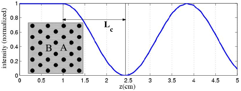
Figure 4: Intensity of electric field in the center of the core $A$. The inset shows the cross section of the PCF coupler with the two cores $A$ and $B$.

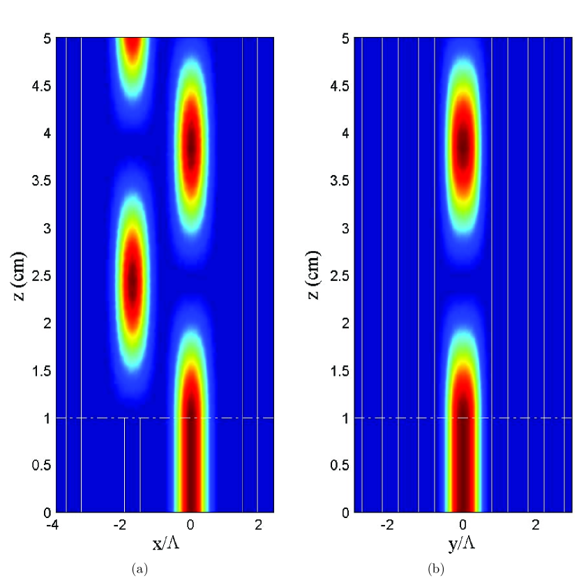
Figure 5: Distribution of electric field intensity (a) in the $xz$ plane at the centers of the fibre cores (b) in the $xy$ plane. The electric field in the $xy$ plane is computed at the center of the core $A$.

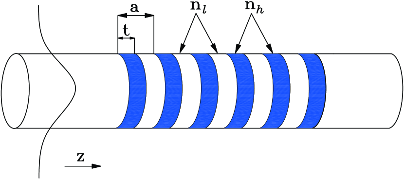
Figure 6: Geometry of the photonic crystal fibre distributed Bragg reflector.

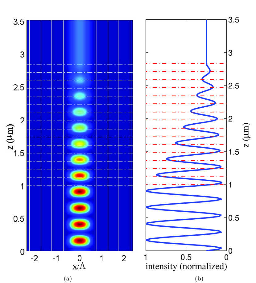
Figure 7: Distribution of electric field intensity (a) on the $xz$ plane at the center of the fibre core and (b) at the center of the fibre core.

References

- [1] Yablonovitch E 1987 Phys. Rev. Lett. 58 2059 – 2062
- [2] John S 1987 Phys. Rev. Lett. 58 2486 – 2489
- [3] Knight J C, Broeng J, Birks T A and Russel P S J 1998 Science 282 1476 – 1478
- [4] Cregan R F, Mangan B J, Knight J C, Birks T A, Russell P S J, Roberts P J and Allan D C 1999 Science 285 1537 – 1539
- [5] Knight J C, Birks T A, Russell P S J and Atkin D M 1996 Opt. Lett. 21 1547 – 1549
- [6] Birks T A, Knight J C and Russell P S J 1997 Opt. Lett. 22 961 – 963
- [7] Russell P S J 2003 Science 299 358 – 362
- [8] Knight J C 2003 Nature 424 847 – 851
- [9] Nielsen M D, Folkenberg J R, Mortensen N A and Bjarklev A 2004 Opt. Express 12 430 – 435
- [10] Birks T A, Mogilevtsev D, Knight J C and Russell P S J 1999 IEEE Phot. Technol. Lett. 11 674 – 676
- [11] Knight J C, Arriaga J, Birks T A, Ortigosa-Blanch A, Wadsworth W J and Russell P S 2000 IEEE Phot. Technol. Lett. 12 807 – 809
- [12] Mortensen N A 2002 Opt. Express 10 341 – 348
- [13] Mangan B J, Knight J C, Birks T A, Russell P S J and Greenaway A H 2000 Electron. Lett. 36 1358 – 1359
- [14] Saitoh K, Sato Y and Koshiba M 2003 Opt. Express 11 3188 – 3195
- [15] Saitoh K, Sato Y and Koshiba M 2004 Opt. Express 12 3940 – 3946
- [16] Eggleton B J, Kerbage C, Westbrook P S, Windeler R S and Hale A 2001 Opt. Express 9 698 – 713
- [17] Larsen T T, Broeng J, Hermann D S and Bjarklev A 2003 Electron. Lett. 39 1719 – 1720
- [18] Larsen T T, Bjarklev A, Hermann D S and Broeng J 2003 Opt. Express 11 2589 – 2596
- [19] Du F, Lu Y Q and Wu S T 2004 Appl. Phys. Lett. 85 2181 – 2183
- [20] Alkeskjold T T, Lægsgaard J, Bjarklev A, Hermann D S, Anawati, Broeng J, Li J and Wu S T 2004 Opt. Express 12 5857 – 5871
- [21] Limpert J, Schreiber T, Nolte S, Zellmer H, Tünnermann A, Iliew R, Lederer F, Broeng J, Vienne G, Petersson A and Jakobsen C 2003 Opt. Express 11 818 – 823
- [22] Saitoh K and Koshiba M 2001 J. Lightwave Technol. 19 405 – 413
- [23] Peng S T, Tamir T and Bertoni H L 1975 IEEE Trans. Microw. Theory Tech. MTT-23 123 – 133
- [24] Tamir T and Zhang S Z 1996 J. Lightwave Technol. 14 914 – 927
- [25] Akbari M, Shahabadi M and Schünemann K 1999 Progress in Electromagnetic Research PIER-22 197–212
- [26] Akbari M, Schünemann K and Burkhard H 2000 Opt. Quant. Electron. 32 991 – 1004
- [27] Lin C H, Leung K M and Tamir T 2002 J. Opt. Soc. Am. A 19 2005 – 2017
- [28] Yan L B, Jiang M M, Tamir T and Choi K K 1999 IEEE J. Quantum Electron. 35 1870 – 1877
- [29] Shahabadi M and Schünemann K 1997 IEEE Trans. Microw. Theory Tech. 45 2316 – 2323
- [30] Zhang S H and Tamir T 1996 J. Opt. Soc. Am. A 13 2403 – 2413
- [31] Dabirian A, Akbari M and Mortensen N A 2005 Opt. Express 13 3999 – 4004
- [32] Faria J A B 1993 Multiconductor Transmission-Line structures-Modal Analysis Technniques (New York: John Wiley & Sons, Inc.)
- [33] Desoer C A and Kuh E S 1969 Basic Circuit Theory (New York: McGraw–Hill)
- [34] Dabirian A and Akbari M 2005 J. Electromagn. Waves Appl. 19 891 – 906
- [35] Brandbyge M, Sørensen M R and Jacobsen K W 1997 Phys. Rev. B 56 14956 – 14959
- [36] Zhi W, Guobin R, Shuqin L and Shuisheng J 2003 Opt. Express 11 980 – 991
- [37] Slang M M, Tamir T and Zhang S Z 2001 J. Opt. Soc. Am. A 18 807 – 820
- [38] Yokouchi N, Danner A J and Choquette K D 2003 IEEE J. Sel. Top. Quantum Electron. 9 1439 – 1445
- [39] Song D S, Kim S H, Park H G, Kim C K and Lee Y H 2002 Appl. Phys. Lett. 80 3901 – 3903
- [40] Coldren L A and Corzine S W 1995 Diode Lasers and Photonic Integrated Circuits (New York: John Wiley & Sons, Inc.)
- [41] Lee K H, Baek J H, Hwang I K, Lee Y H, Ser J H, Kim H D and Shin H E 2004 Opt. Express 12 4136 – 4143