Competition of Languages and their Hamming Distance

Abstract

We consider the spreading and competition of languages that are spoken by a population of individuals. The individuals can change their mother tongue during their lifespan, pass on their language to their offspring and finally die. The languages are described by bitstrings, their mutual difference is expressed in terms of their Hamming distance. Language evolution is determined by mutation and adaptation rates. In particular we consider the case where the replacement of a language by another one is determined by their mutual Hamming distance. As a function of the mutation rate we find a sharp transition between a scenario with one dominant language and fragmentation into many language clusters. The transition is also reflected in the Hamming distance between the two languages with the largest and second to largest number of speakers. We also consider the case where the population is localized on a square lattice and the interaction of individuals is restricted to a certain geometrical domain. Here it is again the Hamming distance that plays an essential role in the final fate of a language of either surviving or being extinct.

Keywords: evolution of languages, population dynamics, bitstring models

1 Introduction

Evolution of language attracts the attention of linguists, neuro- and computer-scientists, as well as physicists. It concerns basic questions as the origin of speech, the role of mimicry and movement, fine and rapid motor control, but also language development [1]. Language development refers to the individual level during childhood, but also to language evolution of mankind on a global scale. The evolution of a single language as a function of time may refer to a transformation of this language, say from ancient Latin to modern Italian.

When we talk about language evolution or language development in this paper, we address the spreading, competition, extinction and dominance of languages as a function of mutation and adaptation rates that characterize the individual speakers. Similarly to the evolution of cultural traits for various cultural features to a homogeneous or multicultural polarized state [2], one may ask here how an initially multilingual population evolves: do the languages of individuals converge to a common “lingua franca” in the very end, or is a fragmentation into many coexisting language clusters the final state?

From daily-life experience it is intuitively clear that opposing tendencies are at work: the convenience of having one common language and the definition of national identity via language favor language dominance or fragmentation, respectively. However, when it comes to predictions for one of those scenarios, specific mathematical modelling is needed to understand the transition between dominance and fragmentation as various parameters change, and to predict more specific features of this transition, e.g. whether it is sharp or smooth.

Evolutionary models for language development have only recently been proposed. There are macroscopic models, formulated in terms of differential (rate) equations for population rates (that speak a certain language)[3]. They are macroscopic in the sense that the fate of individuals is completely ignored for language competition and the population rates refer to average quantities. Stauffer and Schulze [4] performed microscopic simulations of language populations. Individuals inherit their mother tongue from their parents, with a certain amount of mutation. They change (adapt, replace) their language during their lifespan, pass on their language to offspring, again with a certain amount of mutation, and finally die. The time evolution of the population follows a Verhulst dynamics until a stable population size is achieved. The individuals are described by bitstrings which code for their language. There are as many different languages possible in the population as bitstring states, that is $2^{n}$ if $n$ is the length of the string.

In this paper we extend the simulations of Schulze and Stauffer to include the measurement of the Hamming distance between the dominating languages. We also generalize their model to implement the Hamming distance in the interaction of individuals. A language replacement is more likely to happen between languages with small Hamming distance than with large one. Moreover, we locate the population on a network (so far on a square lattice, for simplicity) to simulate the influence of neighborhood. The neighborhood can refer to “external” (geometric) or “internal” (social) space. Individuals influence their various languages within a certain neighborhood, the so-called interaction range.

In the simulations so far [4], all positions of bits within a bitstring are on an equal footing; we do not attempt any mapping from features of languages like grammar, syntax, vocabulary, to particular sequences of bits. Therefore, although languages differing by just one bit in their bitstring description would probably more appropriately be called dialects, our model is too rough for such distinctions. In principle, it would be possible to reserve a certain part of the bit-sequence to grammatical features, others to the vocabulary and so on; the rules for changing the bits would then depend on the position in the string. Such generalizations are left for the future.

The paper is organized as follows. In section 2 we present our model, in section 3 we summarize the results of the simulations and give a final outlook in section 4.

2 The Model

In this paper we consider extensions of the model presented in [4]. The first one deals with a population with random interactions, independent of the spatial location of individuals, the second one with a population living on a square lattice with free and periodic boundary conditions, and a finite interaction range.

2.1 Language population with random interactions

We consider a population of individuals described by bitstrings of length $n=32$; as argued in [4], $n=30$ is already considered sufficient for language simulations. The position of a bit inside the string is given no specific meaning apart from its use as coordinate to specify a certain language. All $2^{n}$ possible different realizations of a bitstring are called languages. Two different bitstrings are thought to represent different languages, even if they differ just by one bit.

The number of individuals, i.e. the population size, evolves according to a Verhulst dynamics. At each time step, an individual can either die, or live and give birth to one offspring with probability $\alpha$. Here we have chosen $\alpha=1$ in all simulations. This means that an individual has one offspring once it survives at time step $t$. Death occurs due to competition for resources, so that the probability for dying is chosen proportional to the population size $N$ at time $t$; that is, $\beta\cdot N(t)$. The population size effectively follows a dynamics determined by

$$\frac{dN(t)}{dt}\;=\;\alpha\cdot(1-\beta N(t))\cdot N(t)\;-\;\beta N(t)^{2}$$ (1)

The gain term (first term) on the r.h.s.​​ of Eq.(1) reflects the rule that at time $t$, only that fraction of the population which does not die at that time-step [that is, $(1-\beta N(t))$], can have an offspring, with probability $\alpha$. The loss term (second term) is quadratic in $N(t)$ to implement the competition for resources: death occurs with a probability proportional to the current population size. A stationary population size $N_{0}$ is obtained for $\alpha$ and $\beta$ chosen such that $N_{0}\;=\;\frac{\alpha}{(1+\alpha)\cdot\beta}$. In the simulation, we chose $\alpha$ and $N_{0}$ as independent parameters, and adjusted $\beta$ accordingly.

As offspring are born, they inherit their “mother” tongue from their parent (parent in the singular, because, for simplicity, we consider asexual reproduction within this model; sexual reproduction would offer the interesting option for offspring to grow up bilingually [5].) With a probability $p$, the language of a newly-born can undergo a mutation, in which one randomly chosen bit is switched from the value inherited from the parent.

So far the model is similar to genetic models used in a biological context, e.g. in the context of aging, in which individuals are born and die while their genes suffer from (deleterious) mutations. In contrast to genes, however, languages can be completely exchanged by their speakers during lifetime. It is not unusual for speakers of a language minority to change their language to that spoken by the majority of population. To model this behavior, an individual who speaks a language shared by a fraction $x$ of the population, can change its language with probability $q\cdot(1-x)^{2}$ to the language of a randomly chosen individual. The parameter $q$ is called the language change parameter. (Note that the notation here for $q$ is different from that in [4].)

Large populations (strictly speaking, large population densities) usually increase the social pressure. Since it is often the social pressure that leads to a language switch, we further multiply $q\cdot(1-x)^{2}$ by $N(t)/N_{0}$ so that the pressure is smaller in the expansion period than in the stable state. The power of $(1-x)$, here chosen as two, can be used to tune the “social pressure”. The larger the exponent the less likely a switch in language of the minority speakers. The effective exponent is actually three, because there is also the possibility that the randomly chosen person whose language is the new candidate for a switch, speaks the same language as the original one.

We extended the simulations of Schulze and Stauffer to measure the Hamming distance between languages. (The Hamming distance between two bitstrings is defined as the number of bits at corresponding positions inside the string, by which the two strings differ.) The Hamming distance is a quantitative measure for how much two languages differ. In this paper we are interested in the Hamming distance between the languages with the largest and the second largest number of speakers. Are these languages similar or very different? Moreover, this measure allows to implement and model language barriers of the type that an Italian is more likely to learn French than Chinese, since the learning effort is proportional to the difference. In an extended version of the former model, that we consider below, an individual with language A switches to language B of another individual, randomly chosen from the population together with $m-1$ other individuals, but distinguished by the fact that language B comes closest to A in terms of the Hamming distance. In case that several candidates come closest to $A$, because they have the same shortest distance to $A$, we take the first one out of the selection process. For $m=1$ the model reduces to the former one. Again the switch is not deterministic, but happens with probability $q\cdot(1-x)^{2}\cdot N(t)/N_{0}$.

To summarize: the parameters that govern language dynamics in these models, are the number $n$ of bits in a string coding a specific language, the birth rate $\alpha$ for offspring, the asymptotic population size $N_{0}$ (implicitly determining the death rate $\propto\beta$), the language mutation rate $p$, the language change parameter $q$, and, in the extended version, the number $m$ of individuals that is analyzed with respect to their similarities, before the individual decides about a switch.

So far, all $2^{n}$ different languages, described by the state space of bit strings, are treated on an equal footing. Effective weights come only from their number of speakers, but no intrinsic fitness was assigned to languages within these models.

2.2 Language population on a lattice

In this model, the “language population”, is placed on a square lattice. This assignment allows the description of interactions that depend on the distance. The distance may either represent the distance in Euclidean space or in internal space, where “internal” can be e.g. “social”. The distance in Euclidean space plays a role for modelling situations in which the pressure on people for learning a foreign language is small when they live in the center of a large country rather than at the border with another country. Due to modern communication channels, this distance has lost its meaning to a certain extent, because an individual, exposed to a foreign country, can keep and speak its mother tongue with friends via phone or internet. In this case, the friends would represent the nearest neighbors on a square lattice in internal space. Of course, the regular features of a square lattice look unrealistic as compared to network topologies like small-world, hierarchical, or scale-free networks, but as we shall see below, we use the regular features only for defining the interaction range. Out of this interaction range, randomly selected sites are then chosen for language comparison to decide which language is taken over.

For simplicity we suppress the aspect of population evolution: there are no birth or death rates, and each lattice site is always occupied. To simplify the wording, from now on we will no longer distinguish between an individual or speaker who speaks a certain language, and the language itself, since individuals are exclusively specified by their language (at a given site.) At each time step, each individual can change its language with probability $q$, to a different one chosen from those within a given interaction range. The interaction range is defined as a rectangular region centered at the individual. The half-height $\Delta i$ and the half-width $\Delta j$ of this region are parameters of the simulation. Both periodic and non-periodic boundary conditions are implemented. In order to choose the language to which an individual switches, we use a rule similar to the former model: the individual randomly selects $m$ languages out of the interaction range, and then chooses the one that is closest to its own in terms of Hamming distance. Due to the random selection within the interaction range, we actually use the regular features of the square lattice in a very weak form. The selected candidates may be nearest, next-to-nearest neighbors or the like. The finite size of the square lattice enters in case of non-periodic boundary conditions via the interaction range that is chopped to fit into the simulation area when it touches the boundary. In case of periodic boundary conditions, lattice sites on opposite boundaries are identified as usual, so that the interaction range is embedded in a torus.

In addition to language switches, at each time-step individuals mutate their language with probability $p$ by a one-bit mutation, as in the previous model by Schulze and Stauffer. Due to the localization of speakers, the simulations amount to an animation that shows the state of the language lattice at each time step. Mechanisms such as language dominance or cluster formation are easily visualized this way. (For language simulations on lattices see also [6].)

3 Results

3.1 Language population with random interactions

We performed simulations for population sizes $N_{0}$ ranging from 1000 to 100 000 (in factors of 10), for mutation rate and language change parameters from $0$ to $1$ in various steps (see below), and for lengths $n$ of the bitstrings with $16\leq n\leq 32$ in steps of $1$. We considered cases with language switch independent and dependent on the Hamming distance ($m=1$ and $m=4$, respectively, in the notation of the previous section.) In order to check the dependence on the initial conditions, we focused on two cases; in the first case we studied one initial speaker with language zero and let the population grow until it reached its stable size; in the second case, the population was initially comprised of the asymptotic number $N_{0}$ of individuals, half of them speaking language $00_{(16)}$, and the other half speaking $\mbox{FF}_{(16)}$. Here we are using a common notation for hexadecimal numbers, that is $00_{(16)}$ $=0\cdot 16^{0}+0\cdot 16^{1}=0$, $\mbox{FF}_{(16)}$ $=15\cdot 16^{0}+15\cdot 16^{1}=255$. In the bitstring, coding for language $255_{(10)}$ $\equiv\mbox{FF}_{(16)}$, $n-8$ zero-bits are followed by $8$ one-bits, where $n$ was usually chosen as $32$. We were interested in this latter case to see whether competition of two equally represented languages leads to the dominance of one of them or to the rise of a third one.

Each simulation was run for $1000$ time-steps, and the following parameters were recorded every $10$ steps

• the number of individuals in the population $N(t)$

• the number of languages with more than ten speakers $n_{l}$

• the fraction of the population speaking the language of the majority $f_{0}(t)$

• the fraction of the population speaking the language with the second largest number of speakers $f_{1}(t)$

• the Hamming distance between the languages with the two largest numbers of speakers $d_{0}(t)$

After the last time-step of each simulation, we recorded these parameters together with the bitstrings for the two “largest” languages in order to measure their Hamming distance. As it turned out, already after less than a hundred iterations, $N(t)$, $n_{1}$, $f_{0}(t)$, $f_{1}(t)$, and $d_{0}(t)$ reached their stable values in both cases, $m=1$ and $m=4$, so that $1000$ time-steps were sufficient for the population to stabilize in these properties.

3.2 Language switch independent of the Hamming distance

In our simulations, after $1000$ time-steps, we observed essentially two scenarios. In the first one the language population is characterized by dominance of one language that comprises the largest part of the population, while the rest of the population is scattered between many small languages. The second scenario is fragmentation, a state in which no language has significantly more speakers than the others. The dominance of languages is accompanied by the fact that in this phase the Hamming distance between the two largest languages is usually equal to $1$, that is, the smallest possible value for two different languages. Therefore, an even larger part of the population speaks almost the same language. In the absence of a dominant language, the Hamming distance between the two largest languages is large, about $16$ (for $n=32$) in our simulations.

The way we have implemented the switch to another language supports language dominance, since speakers of a minority language have a high probability to switch to the majority language when they randomly select the language to which they switch. On the other hand, mutation acts toward fragmentation by spreading the speakers in language space. The result of these competing tendencies can hardly be predicted intuitively. It was therefore analyzed in the simulations. The transition between these two cases is sharp, it looks like first order, and, all other parameters fixed, occurs at a critical value of the mutation rate, $p_{0}$. This can be seen, for instance, in Figure 1,

a.

b.

Figure 1: Dependence of the relative size of the largest language on the mutation rate $p$, for various language change parameters $q$. $N_{0}=$100 000, $n=32$. a. Initially just one speaker of language zero. b. Initially $N_{0}$ individuals, speaking languages $00_{(16)}$ and $\mbox{FF}_{(16)}$ (in hexadecimal) equally.

where the relative size of the largest language is large for $p<p_{0}$ and almost zero for $p>p_{0}$ (in Figure 1a the initial population contained only one speaker of language zero, while it had $N_{0}$ speakers in Figure 1b, half speaking language $00_{(16)}$, half $\mbox{FF}_{(16)}$. Therefore, initially, also in the latter case only the eight most-right bits out of the $32$ are ”used”, i.e. they are one, but later, during the simulation, all other $24$ bits may be switched to one due to the random mutations.) As mentioned in [4], we also observed that at values $p$ close to $p_{0}$, it may be possible to obtain both dominance and fragmentation in different runs of the simulation.

The position $p_{0}$ of the phase transition depends on a number of factors. Since the mutation rate $p$ acts toward fragmentation, while the language change parameter $q$ acts toward dominance, $p_{0}$ will obviously depend on $q$ as it is already seen from Figure 1. Figure 2

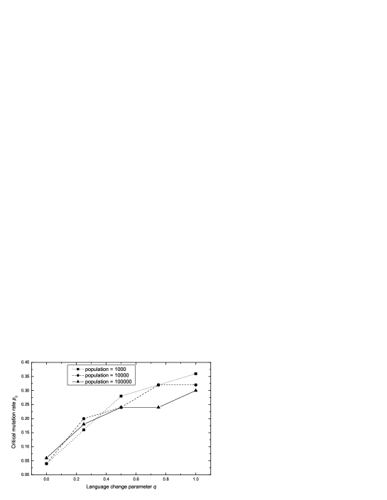
Figure 2: Dependence of the critical mutation rate $p_{0}$ on the language change parameter $q$, at different population sizes; initially one speaker of language zero, $n=32$.

shows the dependence of the critical mutation rate on the language change parameter $q$ for different population sizes. As observed in [4], $p_{0}$ also depends on the size of the population, although the tested range was varied only between $1000$ and 100 000 individuals, while in [4] it was varied up to $10^{7}$.

Figure 3: Dependence of the critical mutation rate $p_{0}$ on the language change parameter $q$. $N_{0}=$100 000, $n=32$.

The location of the phase transition also depends on the initial conditions of the simulation. In case the initial population starts with many speakers of two evenly represented languages, here chosen as $00_{(16)}$ and $\mbox{FF}_{(16)}$, the critical mutation rates are larger than in the case of initially one individual, especially for large values of the language change parameter $q$, Figure 3. This effect can be explained by the fact that it is harder to break the initially big domains of languages, in contrast to the single speaker of language zero in the other case.

As we have seen above, in the case of dominance, one language has many more speakers than all the others. Due to mutation, a fraction of these speakers switches at each time step to a language that differs from the largest one by a single bit. In the stationary state, the number of speakers who switch to such a language, is approximately equal to the number of speakers who switch back to the largest population due to the option of a language switch. Since in this realization a single mutation cannot change the language by more than one bit, languages that differ by two or more bits from the largest one are disfavored.

The effect is seen in measurements of the Hamming distance (number of different bits) between the two largest languages. It is equal to one (rarely two) before the transition $(p<p_{0})$, and large (around $16$ for $n=32$ bits per language) after the transition. Figure 4

a.

b.

Figure 4: Phase transition in the Hamming distance between the two largest languages. The asymptotic population size is $N_{0}=$100 000 in both cases, $n=32$. a. Initially one speaker of language zero. b. Initially $N_{0}$ speakers evenly distributed among languages $00_{(16)}$ and $\mbox{FF}_{(16)}$ (hexadecimal.)

shows this effect also in dependence on the initial conditions. The coincidence of the transition in the Hamming distance with the one in the relative size of the largest language can be seen in Figure 5.

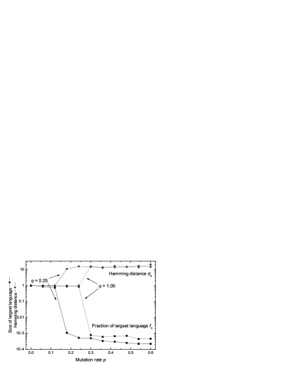
a.

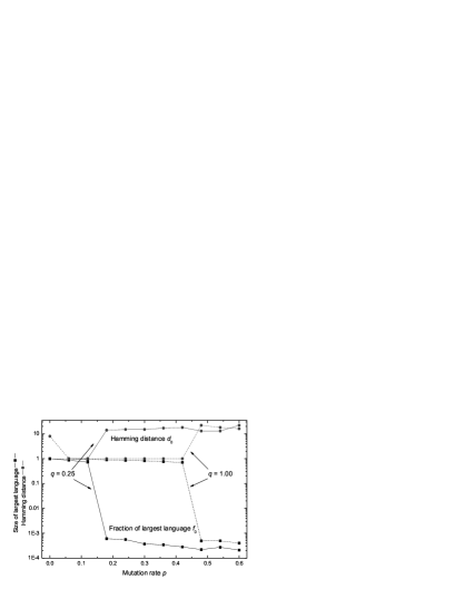
b.

Figure 5: Coincidence of phase transition in Hamming distance between the two largest languages, with the one in the relative size of the largest language. The asymptotic population size is $N_{0}=$100 000. The solid line corresponds to $q=0.25$, and the dashed one to $q=1.00$. a. Initially one speaker of language zero. b. Initially $N_{0}$ speakers evenly distributed among languages $00_{(16)}$ and $\mbox{FF}_{(16)}$ (hexadecimal.)

Moreover, we observed that in case of dominance, the final largest language is one of the initial languages, possibly with one or two bits mutated. In the case where initially there is only one speaker of language zero, the final dominant language is thus expected to be language zero or a one- or two-bit mutation of it. Initial conditions with languages $00_{(16)}$ and $\mbox{FF}_{(16)}$ lead to a final dominant language that is one of the initial two, up to a few mutations. Therefore we can neither describe the evolution from ancient Latin to modern Italian as long as one-bit mutations are unbiased, nor the creation of English out of ancient French and ancient German within this model, as long as we only allow one-bit mutations and complete switches, but no “superposition” of languages in analogy to the mixing of genes in biology (cf. [7] for a proposal of a model in this direction.)

The previous results were obtained by using $n=32$ bits per language. The position of the phase transition is largely independent of the bitlength $n$. This can be expected because the language switch, which is opposing dominance, is itself independent of $n$. The critical mutation rate for various bitlengths is plotted in Figure 6, for the case where in the initial state there was one speaker of language zero. We observed the same effect when we had in the initial state $N_{0}$ speakers equally spread among two languages.

In view of computational aspects we remark that bitstrings as long as $32$ bits (providing a large language space, but for the case of less large population size), were efficiently treated by using a hash-table, so that the complexity of the simulation was $O(N)$, i.e. linear in the population size.

Figure 6: Dependence of the critical mutation rate on the bitlength $n$. Asymptotic population size is $N_{0}=$10 000, and initial state contained one speaker of language zero. $q=0.25$.

3.3 Language switch determined by the Hamming distance

In case the language switch depends on the Hamming distance, as described in section 2.1, the formation of language clusters is more favored than the dominance scenario as compared to the previous model $(m=1)$, since each individual is more conservative in changing its language. Therefore the sharp transition that was observed for $m=1$ between dominance and fragmentation is smoothed out, see Figure 7.

a.

b.

Figure 7: Smooth crossover in case of Hamming-distance dependent language change (for $m=4$.) Asymptotic population size is $N_{0}=$ 100 000 in both cases. a. Initially one speaker of language zero. b. Initially $N_{0}$ speakers evenly distributed among languages $00_{(16)}$ and $\mbox{FF}_{(16)}$ (hexadecimal.)

Moreover, the dependence on the initial conditions is less strong than before, there is no noticeable difference between the evolution for one or two initial languages, cf. Figures 7a and 7b. This supports the idea of the previous subsection that the dependence on the initial conditions is related to the language dominance, and since dominance in this model is disfavored, the influence due to dominance should be less visible.

The crossover from dominance to fragmentation is still seen as a sharp transition in the Hamming distance between the two largest languages. As it is seen from Figure 8,

a.

b.

Figure 8: Phase transition in the Hamming distance between the two largest languages, in the case of Hamming-distance dependent language change (with $m=4$.) Values are averages of two runs for each $p$. Asymptotic population size is $N_{0}=$ 100 000 in both cases. a. Initially one speaker of language zero. b. Initially $N_{0}$ speakers evenly distributed among languages $00_{(16)}$ and $\mbox{FF}_{(16)}$.

the Hamming distance is equal to one up to a certain critical mutation rate $p_{0}$ and then rises rather abruptly to values larger than $10$. Again, the position of $p_{0}$ is relatively independent on whether there were initially one or two languages.

We also observed a large variation of the Hamming distance for different runs at the same values of the parameters; changes as high as 30% were observed in the case of fragmentation.

3.4 Language population on a lattice

In this paper we report on results of language evolution on a lattice that allow a visualization of the results, that is, we made snapshots of the language population on the square lattice after each iteration. The simulations were performed on a square lattice of size $400\times 400$ with free boundary conditions, $n=16$ bits, mutation rate $p=0.01$, language change rate $q=0.50$, and interaction range $41\times 41$. The number of individuals considered for language change was $m=2$. As it turned out in the simulations, the parameters $p$ and $q$ of language mutation and language switch are of little relevance for the outcome compared to the initial conditions, in contrast to the simulations of the $m=1$ model. Because of the similarity with the $m=4$ model of the previous section, it is not surprising that we found a smooth crossover from the dominance scenario, in which only a few languages survive, to the complete fragmentation. Note that the $m=4$ model and the $m=2$ lattice population essentially differ by the location of the interaction range, here centered at an individual and extended to a finite (possibly small) subset of the lattice in its neighborhood. The former simulation was non-localized, i.e. any subset of $m$ speakers could be selected from the whole population. This difference is probably responsible for the stronger dependence on the initial conditions that is observed here: when the mutation rate is chosen small enough and the language change parameter large enough to form stationary language clusters, the number of such clusters and their location and shape are less likely “washed out” by random interactions, but determined by the initial conditions of the simulation.

Based on the description of the model of section 2.2, a few general features of these simulations can be deduced. It is seen in Figure 9

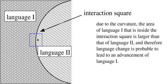
Figure 9: Explanation of instability of curved borders in the lattice simulation.

that the interface between two languages is only stable if it is straight (if $q>0$): an individual placed on the border will probably change its language to the one that is predominant within the interaction range centered at it. A curvature in the interface will make the population on the concave side of the curvature to have less speakers within the interaction range than the population on the other side; therefore, the former is disfavored with respect to the latter language. Moreover, by this argument it can be deduced that any cluster of one language completely surrounded by sites with a different language will not survive; due to the rule described above, it will shrink continuously, until it becomes smaller than the interaction range; in this case it quickly fades away as the ratio of the perimeter to the area of the interaction range becomes larger and larger. This process can be seen in simulation snapshots. In Figure 10

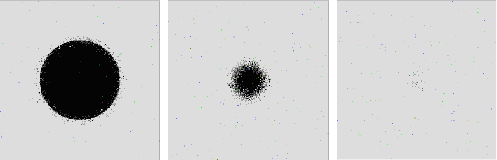
Figure 10: Simulation of a language surrounded by another language, in which the former disappears.

we see the time evolution (from left to right) of how a disk of one language initially surrounded by a different language eventually shrinks to zero. This fate of a language island would change in an extended model, in which inhabitants of the island can communicate (via internet, phone, satellite-TV) with remote speakers of their own language.

In Figure 11

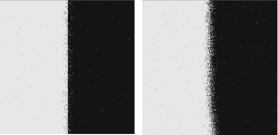
Figure 11: Simulation of stable border between two languages.

we see a stable coexistence of two languages across a straight border, with an inter-penetration depth that is determined by the size of the interaction range. The figure on the left is taken soon after the beginning of the simulation, while the one on the right shows the stationary state that is finally reached. In an extended version of this model, one could imitate different language policies in neighboring countries, leading to asymmetrical penetration depths.

Beyond the coexistence of two languages along straight borderlines, we simulated the coexistence of three languages, Figure 12 (again, time goes from left to right.) The initial conditions had one language, in the shape of a square, in the middle of a “gradient” of languages, where the languages were the same along horizontal lines, and changing from line to line. The gradient of languages started from language $3500_{(16)}$ (again in hexadecimal notation) at the top of the simulation space, and the language code (in terms of integers) increased by one each line, up to $CB00_{(16)}$ at the bottom with $n-16$ leading zero bits. Due to this gradient, none of the languages outside the square is strong enough, and the engulfed language can “capture” the middle of the simulation lattice. The gradient is transformed into clusters from which only the upper and the lower two remain stable (as indicated in the outermost right picture in Figure 12. Note that similar shades of grey at the top and bottom of the picture do not necessarily correspond to similar languages.)

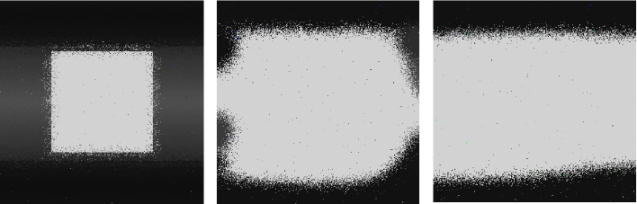
Figure 12: Simulation of the coexistence of three languages.

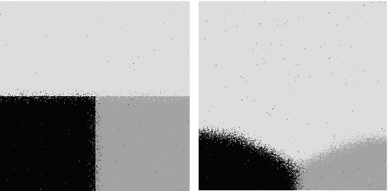
Figure 13: Simulation of three languages coexisting as a metastable state.

The language evolution presented in Figure 13 (time from left to right) shows how a metastable state is reached, where three languages survive. The state shown in the right picture survives for some time, but ultimately the upper language is able to completely eliminate the lower two ones, because it initially occupies twice the area of the other languages, and due to the interaction rules the probability for switching to another language is proportional to the area this language occupies.

More interesting in this case is that the final state of the simulation depends on the Hamming distance between the three initial languages. In Figure 13, the Hamming distance between any two of the initial languages was equal to two. By changing only the bitstring describing the upper language, so that the Hamming distance between it and the lower-left one was equal to one, while the distance to the lower-right language became three, we obtained the evolution from Figure 14, where in the final state, two languages survived instead of one.

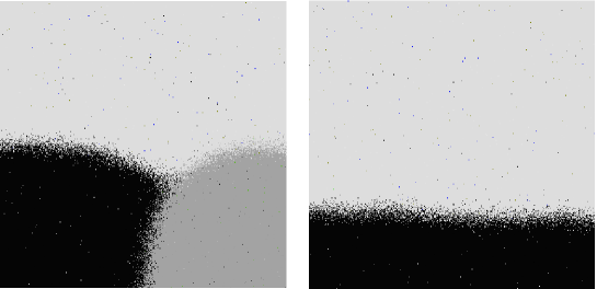
Figure 14: Simulation showing dependence of outcome on the Hamming distance between the languages.

If the language in the lower-left quarter of the plane is close in terms of the Hamming distance to the language in the upper half-plane, these two eliminate the third language and coexist as a stable state. As explanation for the extinction of the third language in Figure 14, we note that the upper and lower-left coincide within the range of mutations if the Hamming distance is small. An individual “living” at the confluence of the three languages, is going to be biased toward changing its language to the upper population, because that is predominant within its interaction range. In the next time-step, only a one-bit mutation can make this individual switch to the lower-left language, while one time-step is not enough for it to mutate to the lower-right one. In this way, the lower-left language has a slight advantage with respect to the lower-right one, and we obtain the observed outcome. Stated differently, the upper and lower-left languages coincide within the typical size of mutations; by arguments analogous to those of Figure 10, the lower-right language then fades away.

It would be expected that even for larger values of the Hamming distances, for instance, when the upper and the lower-left languages differ by 2 bits, while the difference between the upper and the lower-right languages is 3 bits, the lower-left language would still have a slight advantage, and would eventually overrun the lower-right one. That is indeed observed in simulations. As expected, however, the time needed to reach the final state is longer than in the previous case.

4 Summary and Outlook

4.1 Language population with random interactions

In the original model of Schulze and Stauffer, we observe sharp transitions between phases of language dominance and language fragmentation, and along with this, transitions between small and large Hamming distances between the two largest languages, both types of transitions driven by the mutation parameter $p$ for given language change parameter $q$ and total size $N$, or, alternatively, driven by $q$ for given $p$ and $N$. The precise location of the critical mutation rate depends on the language change probability $q$, the initial conditions and the population size. In the extended model ($m=4$), the transition between the dominance and fragmentation phases is smoothed out, since the switch to another language happens more conservatively; at the same time, the transition in the Hamming distance is still sharp. For $m=4$, the transitions are less dependent on the initial conditions, because dominance of a certain language is less favored than in the original model.

In particular, we found in the scenario of language dominance that a population evolution starting with one speaker initially, does not alter the initial language if the population has reached its stable size and prefers one dominant language. This is not surprising although unrealistic, because the one-bit mutations happen randomly and the switches favor dominance. For a stable population size and two coexisting languages in the beginning, the evolution favors a dominant language in the end that is one of the coexisting initial languages rather than a “superposition” of both.

4.2 Language population on a square lattice

The evolution of the language population on a square lattice was visualized as a function of time. The square lattice was only used to define the interaction range. A number of $m$ speakers was randomly chosen out of the interaction range and the one with the smallest Hamming distance to a given language was used in the switch with probability $q$. Here we found a sensitive dependence on the initial conditions, and depending on the mutual Hamming distance, an initial set of two or three coexisting languages turned out to give unstable, stable or metastable configurations. Here further investigations are needed to predict the stability behavior beyond the level of numerical evidence.

The models considered in this paper allow for several extensions. Biased mutations (with $r\geq 1$ bits mutated in a single event) are a necessary condition for modelling language development from its ancient to the modern version of the language. In the so-called language change, we considered only a full replacement of one language by another one, randomly chosen. Neither the random one-bit mutations nor the full switches will ever mimic the development of English out of ancient French and ancient German. On a longer time-scale, the bitstring dynamics for languages should imitate the interaction dynamics of parent genes in sexual reproduction, resulting in the genes of their offspring. A description of this dynamics would need, however, a deeper understanding of language evolution from the viewpoint of linguistics and a mapping between the bits and realistic traits or features of languages.

5 Acknowledgements

It is a pleasure to thank D. Stauffer for drawing our attention to the topic of language competition.

References

-
[1]
D.M.Abrams, S.H.Strogatz, Nature 424,
900 (2003)
Y. Bhattacharjee, Science 303, 1326 (2004)
C. Holden, Science 303, 1316 (2004) -
[2]
R. Axelrod. Journal of Conflict Resolution 41, 203 (1997)
R. Axelrod. The complexity of cooperation. Princeton University Press, Princeton, (1997)
M. San Miguel, V.M. Eguíluz, R. Toral, and K. Klemm, 2005, Comp. Sci. Engin. 7, issue 6 (2005), and physics/0507201 - [3] M.A. Nowak, N.L. Komarova and P. Niyogi, Nature 417, 611 (2002) and Science 291, 114 (2001)
-
[4]
D. Stauffer, C. Schulze, Physics of Life Reviews 2, 89 (2005)
C. Schulze and D. Stauffer. Int. J.Mod.Phys.C 16, 781(2005) - [5] J.Mira, A.Paredes, Europhys.Lett.69, 1031 (2005); K.Kosmidis, J.M.Halley, P.Argyrakis, Physica A353, 595 (2005)
-
[6]
M. Patriarca, T. Leppänen, Physica A 338, 296 (2004)
V.M.de Oliveira, M.A.F.Gomes, I.R.Tsang, Physica A (2005), in press, and physics/0505197
V. Schwämmle, Int.J.Mod.Phys.C 16, in press, and physics/0503238 - [7] C.Schulze and D.Stauffer, physics/0502144