Waiting-time distribution for a stock-market index

Abstract

We investigate the waiting-time distribution of the absolute return in the Korean stock-market index KOSPI. We define the waiting time as a time interval during which the normalized absolute return remains continuously below a threshold $r_{c}$. Through an exponential bin plot, we observe that the waiting-time distribution shows power-law behavior, $p_{f}(t)\sim t^{-\beta}$, for a range of threshold values. The waiting-time distribution has two scaling regimes, separated by the crossover time $t_{c}\approx 200$ min. The power-law exponents of the waiting-time distribution decrease when the return time $\Delta t$ increases. In the late-time regime, $t>t_{c}$, the power-law exponents are independent of the threshold to within the error bars for fixed return time.

I INTRODUCTION

In recent decades, the dynamics of stock markets have been studied by a number of methods from statistical physics MA99 ; MA97 ; BP00 ; SO03 ; MS95 ; BS94 ; BA1900 ; MA63 ; FA63 ; GP99 ; GM99 ; LG99 ; GP00 ; SA00 ; BC03 ; LE02 ; LL04 ; LL05 . The complex behaviors of economic systems have been found to be very similar to those of other complex systems, customarily studied in statistical physics; in particular, critical phenomena. Stock-market indexes around the world have been precisely recorded for many years and therefore represent a rich source of data for quantitative analysis. The dynamic behaviors of stock markets have been studied by various methods, such as distribution functions GP99 ; GM99 ; LG99 ; GP00 ; LL04 , correlation functions LG99 ; GP00 ; SA00 , multifractal analysis GD02 ; SK00 ; AR02 ; EK04 ; BE03 ; AI02 ; IA99 ; TP03 ; BE01 ; MA03 ; XG03 ; JWLEE05 , network analysis BC03 , and waiting-time distributions or first-return-time distributions PM96 ; AL04 ; LA04 ; WL02 ; SW04 ; CO04 ; YD04 ; DP05 ; BE05 ; LJ05 ; IT95 ; SG00 ; RS00 .

Waiting-time distributions (wtd’s) have been studied for many physical phenomena and systems, such as self-organized criticality PM96 , rice piles AL04 , sand piles LA04 , solar flares WL02 , and earthquakes SW04 ; CO04 ; YD04 ; DP05 ; BE05 ; LJ05 ; IT95 . Studies of wtd’s have also been performed for many high-frequency financial data sets SG00 ; RS00 ; RS02 ; SG03 ; SK02 ; KK04 . Concepts of the continuous-time random walk (CTRW) have also been applied to stock markets SG00 ; RS00 ; RS02 ; SG03 ; SK02 . A power-law distribution for the calm time intervals of the price changes has been observed in the Japanese stock market KK04 .

In the present work we consider the wtd for the Korean stock-market index KOSPI (Korean Composite Stock Price Index). A waiting time of the absolute return is defined as an interval between a time when the absolute return falls below a fixed threshold $r_{c}$, and the next time it again exceeds $r_{c}$. It therefore corresponds to a relatively calm period in the time series of the stock index. We observed power-law behavior of the wtd over one to two decades in time.

The rest of this paper is organized as follows. In Section II, we introduce the return of the stock index and its probability density function. In Section III, we present the wtd. Concluding remarks are presented in section IV.

II Return of the Stock Index

We investigate the returns (or price changes) of the Korean stock-market index KOSPI. The data are recorded every minute of trading from March 30, 1992, through November 30, 1999 in the Korean stock market. We count the time during trading hours and remove closing hours, weekends, and holidays from the data. Denoting the stock-market index as $p(t)$, the logarithmic return is defined by

$$g(t)=\log p(t)-\log p(t-\Delta t)\;,$$ (1)

where $\Delta t$ is the time interval between two data points, the so-called return time. The logarithmic return $g(t)$ is thus a function of both $t$ and $\Delta t$. In this article we consider the return times $\Delta t=$ 1min, 10 min, 30 min, 60 min, 600 min (=1day), and 1200 min. The normalized absolute return is defined by

$$r(t)=\left|\frac{g(t)-\langle g(t)\rangle}{\sigma(\Delta t)}\right|\;,$$ (2)

where $\sigma(\Delta t)$ is the standard deviation and $\langle\cdots\rangle$ denotes averaging over the entire time series. It is well known that the probability distribution function (pdf) of the return $g(t)$ has a fat tail GP99 ; GM99 . The tail of the pdf obeys a power law,

$$p(x)\sim x^{-(1+\alpha)}\;,$$ (3)

where $\alpha$ is a nonuniversal scaling exponent that depends on the return time $\Delta t$. The cumulative pdf then also follows a power law, such that

$$P(g>x)=\int^{\infty}_{x}p(y)dy\sim x^{-\alpha}\;.$$ (4)

We observed clear power-law behavior in the tail of the pdf. Using least-squares fits, we obtained the power-law exponents $\alpha=3.06(8)$ for $\Delta t=1$ min and $\alpha=3.2(4)$ for $\Delta t=600$ min.

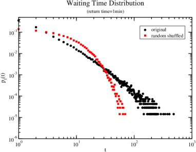
Figure 1: (Color online.) Waiting-time distribution (wtd) of the absolute return for the original data (circles) and the randomly shuffled data (squares) with $\Delta t=1$ min and $r_{c}=1$.

III Waiting-time Distribution

Consider a time series of the absolute return in the stock-market index. The waiting time of the absolute return with a threshold $r_{c}$ is defined as an interval between a time when the absolute return falls below a fixed threshold $r_{c}$, and the next time it again exceeds $r_{c}$. It corresponds to a calm period in the time series of the stock index. The waiting times depend on the threshold $r_{c}$ and the pdf of the absolute return. For small return times, for example $\Delta t=1$ min as in Fig. 1, the absolute return is distributed in a wide range up to $r=500$. However, for large return times, the absolute return is distributed in a narrow range. For large values of the threshold $r_{c}$, the waiting time has very long time intervals. For small values of the threshold $r_{c}$, the waiting time has many short time intervals.

In Fig. 1 we present the wtd of the absolute return for the original data set of KOSPI, together with a randomly shuffled data set. Both sets were analyzed with the threshold $r_{c}=1.0$ for the return time $\Delta t=1$ min. The randomly shuffled data were obtained by exchanging two randomly selected return, repeating the exchanges one hundred times the total number of data points. The wtd of the absolute return shows the power law,

$$p_{f}(t)\sim t^{-\beta}\;,$$ (5)

where the scaling exponent $\beta$ depends on the return time $\Delta t$. However, the randomly shuffled data lose the correlations of the original time series, and the uncorrelated wtd is therefore a simple exponential distribution, $p_{f}(t)=\frac{1}{\langle T\rangle}\exp(-t/\langle T\rangle)$, where $\langle T\rangle$ is the mean waiting time for the given threshold $r_{c}$.

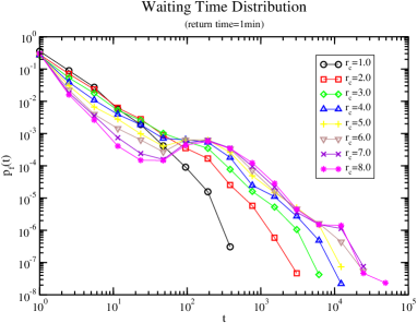
Figure 2: (Color online.) Wtd of the absolute return with $\Delta t=1$ min and several values of $r_{c}$, using the exponential bin plot.

In the wtd in Fig. 1, the data are sparsely distributed in the tail, so it it difficult to measure the scaling exponents of the power law. To calculate the scaling exponents, we have therefore applied the exponential bin plot RZ05 . In the exponential bin plot, we calculate the normalized histogram in bins of exponentially increasing size. If the distribution follows a power law with exponent $\beta$, then the histogram of the distribution also has the same slope $\beta$ in the log-log exponential bin plot: $\log p_{f}(t)=C-\beta\log t$, where $C$ is a constant depending on the return time and the threshold.

In Fig. 2 we present the wtd obtained using the exponential bin plot for the return time $\Delta t=1$ min. We observe clear power-law behavior $t>t_{c}$, where $t_{c}$ is a crossover time. For a small return time, $\Delta t=1$ min, we observe two scaling regimes separated by a crossover time $t_{c}\approx 200$ min. In the log-log plots the curves for $r_{c}=1.0$ to $r_{c}=3.0$ are parallel to each other for $t<t_{c}$, and the slope is measured as $\beta_{1}=1.48(3)$. For $t<t_{c}$ and $r_{c}\geq 4.0$, the wtd decreases quicker than a power law and shows a local maximum around $t=t_{c}$. When we choose a large threshold value $r_{c}$, for example $r_{c}=8.0$, the wtd is still large for small waiting times. This means that the return has clustering behavior, i.e., large absolute returns occur in bursts. For $t>t_{c}$, the wtd shows power-law behavior with similar exponents, regardless of the threshold. When the threshold $r_{c}$ is large, the total number of data points for the wtd decrease. Therefore, the wtd fluctuates much and the uncertainty in the exponent $\beta_{2}$ increases.

The power-law exponents of the wtd are measured by least-squares fits. In Table 1 we present the exponents $\beta_{2}$ for $t>t_{c}$. To measure the exponents, we scaled the wtd by the average waiting time $\langle T\rangle=\int_{1}^{\infty}tp_{f}(t)dt$. We present the wtd scaled by the average waiting time in Fig. 3 for $\Delta t=1$ min. The scaled wtd shows clear power-law behavior. For a given return time, the exponents $\beta_{2}$ are nearly equal within the error bars, regardless of the threshold $r_{c}$. We also observe that the exponents $\beta_{2}$ decrease when the return time $\Delta t$ increases. We obtained the averaged exponents $\beta_{2}$ for the wtd as $\beta_{2}=2.0$ for $\Delta=1$ min, 1.58 for $\Delta t=60$ min, and 1.42 for $\Delta t=600$ min. It is very difficult to identify the origins of the scaling behavior for the wtd. The correlation of the return is one reason of the scaling behavior as shown in Fig. 1, because the shuffled data set destroys the correlation of the time series. The power-law behavior of the probability density function for the absolute return is another reason for the scaling behavior of the wtd. These power-law behaviors may be due to herding behavior of the stock traders and the nonlinear dynamics of the stock market.

Table 1: Critical exponents $\beta_{2}$ for the wtd in the large-$t$ regime.

$r_{c}$	$\beta_{2}$
	$\Delta t=1$ min	$\Delta t=60$ min	$\Delta t=600$ min
1.0	2.04(7)		1.40(5)
2.0	2.0(2)	1.58(7)	1.52(7)
3.0	2.0(1)	1.6(1)	1.36(5)
4.0	2.1(1)	1.58(7)
5.0	2.1(3)	1.46(5)
6.0	2.0(1)
7.0	1.9(2)

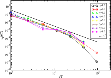
Figure 3: (Color online.) Wtd of the absolute return scaled by the average waiting time $\langle T\rangle$ with $\Delta t=1$ min.

IV Conclusions

We have considered the probability density function of the absolute return and the waiting-time distribution (wtd) with a cut-off threshold. We observed that the probability density function of the absolute return has a power-law behavior. The exponents $\alpha$ decrease when the return time $\Delta t$ increases. We defined the waiting time of the absolute return by the threshold $r_{c}$. The wtd also shows power-law behavior. When the return time $\Delta t$ is less than one day, we observe two scaling regimes, separated by a crossover time around $t_{c}\approx 200$ min.

- (1) R. N. Mantegna and H. E. Stanley, An Introduction to Econophysics: Correlations and Complexity in Finance, Cambridge University Press, Cambridge, 1999.
- (2) B. Mandelbrot, Fractals and Scaling in Finance, Springer, New York, 1997.
- (3) J. P. Bouchaud and M. Potters, Theory of Financial Risk, Cambridge University Press, New York, 2000.
- (4) D. Sornette, Phys. Rep. 378, 1 (2003).
- (5) R. N. Mantegna and H. E. Stanley, Nature 376, 46 (1995).
- (6) J.-P. Bouchaud and D. Sornette, J. Phys. I France 4, 863 (1994).
- (7) L. Bachelier, Ann. Sci. École Norm. Sup. 3, 21 (1900).
- (8) B. Mandelbrot, J. Business 36, 294 (1963).
- (9) E. F. Farma, J. Business 36, 420 (1963).
- (10) P. Gopikrishnan, V. Plerou, L. A. N. Amaral, M. Meyer, and H. E. Stanley, Phys. Rev. E 60, 5305 (1999).
- (11) P. Gopikrishan, M. Meyer, L. A. N. Amaral, and H. E. Stanley, Eur. Phys. J. B. 3, 139 (1999).
- (12) Y. Liu, P. Gopikrishnan, P. Cizeau, M. Meyer, C.-K. Peng, and H. E. Stanley, Phys. Rev. E 60, 1390 (1999).
- (13) P. Gopikrishnan, V. Plerou, Y. Liu, L. A. N. Amaral, X. Gabaix, and H. E. Stanley, Physica A 287, 362 (2000).
- (14) H. E. Stanley, L. A. N. Amaral, P. Gopikrishnan, and V. Plerou, Physica A 283, 31 (2000).
- (15) G. Bonanno, G. Caldarelli, F. Lillo, and R. N. Mantegna, Phys. Rev. E 68, 046130 (2003).
- (16) S. Y. Park, S. J. Koo, K. E. Lee, J. W. Lee, and B. H. Hong, New Physics 44, 293 (2002).
- (17) K. E. Lee and J. W. Lee, J. Kor. Phys. Soc. 44, 668 (2004).
- (18) K. E. Lee and J. W. Lee, J. Kor. Phys. Soc. 46, 726(2005).
- (19) A. Z. Górski, S. Drodz, and J. Septh, Physica A 316, 496 (2002).
- (20) J. A. Skjeltorp, Physica A 283, 486 (2000).
- (21) J. Alvarez-Ramirez, M. Cisneros, C. Ibarra-Valdez, A. Soriano, and E. Scalas, Physica A 313, 651 (2002).
- (22) Z. Eisler and J. Kertesz, Physica A 343, 603 (2004).
- (23) A. Bershadskii, Physica A 317, 591 (2003).
- (24) M. Ausloos and K. Ivanova, Comp. Phys. Comm. 147, 582 (2002).
- (25) K. Ivanova and M. Ausloos, Eur. Phys. J. B 8, 665 (1999).
- (26) A. Turiel and C. J. Perez-Vicente, Physica A 322, 629 (2003).
- (27) A. Bershadskii, J. Phys. A 34, L127 (2001).
- (28) K. Matia, Y. Ashkenazy, and H. E. Stanley, Europhys. Lett. 61, 422 (2003).
- (29) Z. Xu and R. Gencay, Physica A 323, 578 (2003).
- (30) J. W. Lee, K. W. Lee, and P. A. Rikvold. Physica A, in press. E-print: arXiv:nlin.CD/0412038.
- (31) M. Paczuski, S. Maslov, and P. Bak, Phys. Rev. E 53, 716 (1996)
- (32) C. M. Aegerter, K. A. Loricz, and R. J. Wijngaarden, cond-mat/0411261.
- (33) L. Laurson and M. J. Alava, Eur. Phys. J. B 42, 407 (2004).
- (34) M. S. Wheatland and Y. E. Litvinenko, Solar Physics, 211, 255 (2002).
- (35) N. Scafetta and B. J. West, Phys. Rev. Lett. 92, 138501 (2004).
- (36) A. Corral, Phys. Rev. Lett. 92, 108501 (2004).
- (37) X. Yang, S. Du, and J. Ma, Phys. Rev. Lett. 92, 228501 (2004).
- (38) J. Davidsen and M. Paczuski, Phys. Rev. Lett. 94, 048501 (2005).
- (39) A. Bunde, J. F. Eichna, J. W. Kantelhardt, and S. H. Havlin, Phys. Rev. Lett. 94, 048701 (2005).
- (40) M. Lindman, K. Jonsdottir, R. Roverts, B. Lund, and R. Bodvarsson, Phys. Rev. Lett. 94, 108501 (2005).
- (41) K. Ito, Phys. Rev. E 52, 3232 (1995).
- (42) E. Scalas, R. Gorenflo, and F. Mainardi, Physica A 284, 376 (2000).
- (43) M. Raberto, E. Scalas, R. Gorden, and F. Mainardi, cond-mat/0012497.
- (44) M. Raberto, E. Scalas, and F. Mainardi, Physica A 314, 749 (2002).
- (45) E. Scalas, R. Gorenflo, F. Mainardi, M. Mantelli, and M. Raberto, cond-mat/0310305.
- (46) L. Sabatelli, S. Keating, J. Dudley, and P. Richmond, Eur. Phys. J. B 27, 273 (2002).
- (47) T. Kaizoji and M. Kaizoji, Physica A 336, 563 (2004).
- (48) P. A. Rikvold and R. K. P. Zia, Phys. Rev. E 68, 031913 (2003).