Ultracold neutral plasma expansion in two dimensions

Abstract

We extend an isothermal thermal model of ultracold neutral plasma expansion to systems without spherical symmetry, and use this model to interpret new fluorescence measurements on these plasmas. By assuming a self-similar expansion, it is possible to solve the fluid equations analytically and to include velocity effects to predict the fluorescence signals. In spite of the simplicity of this approach, the model reproduces the major features of the experimental data.

Ultracold plasmas are produced from photo-ionized laser-cooled gases killian99 ; kulin00 ; killian01 . In these laboratory plasmas, it is possible to study the kinetics and thermodynamics of multi-component, strongly-interacting Coulomb systems. These systems are characterized by the ratio of the nearest-neighbor Coulomb energy to the average kinetic energy, denoted as $\Gamma=(e^{2}/4\pi\epsilon_{0}d)/(k_{b}T)$, with $d$ being the interparticle spacing.

A new class of ultracold plasma experiments has recently become available in which it is possible to spectroscopically study the plasma ions chen04 ; simien04 ; cummings05 . These plasmas are made using alkaline-earth atoms, because the resonance transition wavelengths of the ions are readily generated using standard laser methods. The spatially-resolved time evolution of the plasma ion temperature and density can be measured using absorption and fluorescence techniques.

These ultracold neutral plasmas are not trapped, although efforts are underway in a few laboratories to trap them. The untrapped plasmas freely expand, and as they expand the density and temperature change radically. Processes of recombination, collisional and thermal ionization, radiative cascade, and adiabatic and evaporative cooling all play important roles in how the system evolves and equilibrates.

A variety of models have been used to investigate the properties of these plasmas robicheaux02 ; robicheaux03 ; kuzmin02a ; kuzmin02b ; mazavet02 ; pohl04 ; pohl05 . One particularly simple isothermal fluid model robicheaux02 has been surprisingly successful in predicting the general features of these plasmas robicheaux03 ; pohl04 ; cummings05 . In this paper we extend this model from the spherically-symmetric Gaussian plasma distributions to Gaussian distributions with elliptical symmetry.

The elliptical symmetry has important experimental advantages. In such systems the plasma expands primarily in two dimensions. The practical advantage is that the density falls more slowly than in the three dimensional case, making it possible to study the plasma for longer times. The Doppler-shift due to the directed expansion of the plasma is also suppressed. It should therefore be possible to study plasma oscillations and heating effects for greater time periods before these oscillations are masked by the directed expansion of the plasma. Finally, if the plasmas are generated from a density-limited neutral atom trap, the elongated symmetry allows a greater number of atoms to be trapped initially, corresponding to a greater column density of plasma ions. This directly increases the visibility of fluorescence and absorption signals.

I Isothermal fluid model

An isothermal fluid model has been presented in the literature robicheaux02 ; robicheaux03 . It successfully reproduces most of the major features of recent experimental work. This model was motivated by trends observed in more sophisticated treatments. The basic ideas of the model will be reviewed here, and an extension to the case of a Gaussian distribution with elliptical symmetry will be presented.

The initial ion density distribution is proportional to the Gaussian distribution of the neutral atom cloud from which the plasma is created. For a spherically symmetric cloud, the initial distribution can be written as $n(r)=n_{0}\exp(-\beta r^{2})$. Because the electrons thermalize much faster than the ions, in this model we take the initial electron density distribution to be the thermal equilibrium distribution, given by the Boltzmann factor:

$$n_{e}(r)=n_{0e}\exp\left[\frac{eV(r)}{k_{B}T}\right]$$ (1)

The lowest temperature plasmas are nearly charge-neutral, and the electron density distribution is approximately equal to the ion density. In this limit, it is shown in robicheaux02 ; robicheaux03 that for a spherically symmetric plasma that to within an arbitrary additive constant the electrical potential energy can be written as

$$eV(r)={k_{B}T}\ln[n(r)/n_{0e}]=-{k_{B}T\beta r^{2}}.$$ (2)

The force is the negative gradient of this potential energy. It is manifestly radial, spherically symmetric, and linearly proportional to the radial coordinate $r$, measured from the center of the plasma. The velocity, which is the time integral of the acceleration, is also linearly proportional to $r$. The consequence is that if the distribution is Gaussian initially, it will remain Gaussian at all times in the expansion.

For the case of non-spherical symmetry, the approach is more or less the same, although the isothermal nature of the plasma has a more restricted meaning. We will take the initial ion density distribution to be Gaussian, symmetric in the $x-y$ plane, and initially elongated in the $z$ direction:

$$n(r,t)=\frac{N\beta_{1}\beta_{2}^{1/2}}{\pi^{3/2}}\exp\left[-(x^{2}+y^{2})\beta_{1}(t)-z^{2}\beta_{2}(t)\right],$$ (3)

The initial conditions are $\beta_{1}(0)=\sigma_{0}^{-2}$ and $\beta_{2}(0)=\alpha^{2}\sigma_{0}^{-2}$, and the parameter $\alpha$ defines the elipticity of the system. The plasma fluid equations for our system are written

$$\frac{\partial n}{\partial t}+\nabla\cdot\left(n\vec{v}\right) = 0$$ (4)

$$\frac{\partial\vec{v}}{\partial t}+\left(\vec{v}\cdot\nabla\right)\vec{v} = \vec{a}.$$ (5)

Following the derivation used in the case of spherical symmetry, the velocity is taken to be $\vec{v}=\gamma_{1}(t)(x\hat{x}+y\hat{y})+\gamma_{2}(t)z\hat{z}$. Inserting this and the density profile of Eq. 3 into Eq. 4 gives

$$2\beta_{2}\left(x^{2}\beta_{1}+y^{2}\beta_{1}-1\right)\left(\dot{\beta}_{1}+2\beta_{1}\gamma_{1}\right)\cdots$$

$$+\;4\beta_{1}\left(z^{2}\beta_{2}-1\right)\left(\dot{\beta}_{2}+2\beta_{2}\gamma_{2}\right) =0.$$ (6)

Because $x$, $y$, and $z$ are independent variables, the only non-trivial solution of this equation is

$$\gamma=-\dot{\beta}/2\beta,$$ (7)

where we have dropped the subscripts because all components have this same form of solution.

Solving Eq. 5 requires a little more care. It is straight- forward to write down the acceleration vector following the derivation of the spherically symmetric case. However, the solution requires that the temperature be isothermal in a given dimension, but anisotropic in space. This condition allows the density distribution to reduce to the proper form in the limiting case of a plasma infinitely long in the $z$ dimension. This decouling requires energy to be conserved separately in the $x-y$ plane and in the $z$ dimension. The plasma equations for these two spaces are now exactly identical and completely separable.

Equation 5 can be re-written (dropping the subscripts) as

$$\dot{\gamma}+\gamma^{2}=2k_{b}T(t)\beta(t)/m,$$ (8)

and the conservation of energy is

$$T(0)=T(t)+\frac{m}{2k_{b}}\frac{\gamma^{2}}{\beta},$$ (9)

where we have neglected the energy due to electron-ion recombination. Equations 7, 8, and 9 are exactly identical to Eq. 2 of Ref. robicheaux02 . Using Eqs. 7 and 9, we now have both $T$ and $\gamma$ in terms of $\beta$. Inserting this into Eq. 8 gives

$$\frac{\ddot{\beta}}{\beta^{2}}-2\frac{\dot{\beta}}{\beta^{3}}+2v_{e}^{2}=0,$$ (10)

where we have made the substitution $v_{e}^{2}=2k_{b}T(0)/m$. The solution to this equation is $\beta_{1}^{-1}=\sigma_{0}^{2}+ct+v^{2}t^{2}$, where $c$ is an integration constant. The constant $c$ must be equal to zero to meet the condition that the ion velocity is initially zero at $t=0$ bergeson03 . The time evolution of the density and velocity functions can now be written as

$$n(\vec{r},t) = \frac{N\exp\left[-(x^{2}+y^{2})/\sigma_{1}^{2}(t)-(z^{2})/\sigma_{2}^{2}(t)\right]}{\pi^{3/2}\sigma_{1}^{2}(t)\sigma_{2}(t)}$$ (11)

$$\vec{v}(\vec{r},t) = v_{e}^{2}t\left(\frac{x}{\sigma_{1}^{2}(t)}\hat{x}+\frac{y}{\sigma_{1}^{2}(t)}\hat{y}+\frac{z}{\sigma_{2}^{2}(t)}\hat{z}\right)$$ (12)

$$\sigma_{1}^{2}(t) = \sigma_{0}^{2}+v_{e}^{2}t^{2}$$ (13)

$$\sigma_{2}^{2}(t) = \alpha^{2}\sigma_{0}^{2}+v_{e}^{2}t^{2}.$$ (14)

We note that for two-dimensional planar Gaussian charge distributions, a closed-form expression for the electric field has been derived bassetti80 ; furman94 . If such a compact analytical solution could be written in the three-dimensional case, it would remove the decoupling constraint that we imposed in order to solve the plasma equations. However, such a solution is not readily apparent.

II Fluorescence signal model

The geometry of our measurements is shown in Fig. 1. In the experiment, the probe laser beam is spatially filtered and focused into the plasma with a confocal beam parameter that is long compared to all plasma dimensions. The position offset of this probe laser relative to the plasma is denoted by the parameter $a$. After the plasma is created, the number of atoms in the column defined by the probe laser beam changes dramatically. When the laser beam passes through the center of the plasma ($a=0$), the number of ions in the beam monotonically decreases. However, if the laser is outside of the initial plasma distribution, as shown in Fig. 1, the number first increases as the plasma moves into the laser beam, and then decreases as the plasma disperses.

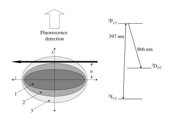
Figure 1: A schematic diagram of the fluorescence measurements. Left — The plasma is initially at a high density, and elongated in the $z$-dimension (labeled region 1). The probe laser is represented by the solid dark arrow parallel to the $z$ axis, displaced by a variable distance $a$. At later times the plasma expands slowly in $z$, but quickly in the $x-y$ plane. Regions 2 and 3 represent the plasma size at later and later times. As the plasma expands, the number of atoms in the column defined by the probe laser changes. Right — a partial level diagram of Ca⁺. The probe laser is locked to the 397 nm resonance transition, and we measure 397 nm light scattered by plasma ions.

The fluorescence signal depends on both the number of ions in the column defined by the probe laser beam (Gaussian beam profile with $1/e^{2}$ radius $w$) and the velocity distribution of the ions in the plasma. Because the laser has a narrow bandwidth, atoms moving at velocities greater than $\sim$9 m/s are Doppler-shifted out of resonance. In this section we will use the results of the previous section to derive an expression for how the plasma ion fluorescence signal should change with time for different values of the offset parameter $a$.

The fluorescence signal $s(t)$ is proportional to the absorption of the probe laser beam. Using Beer’s law and the standard approximation of small optical depth, $s(t)$ can be written as

$$s(t)\propto\int_{\mbox{\footnotesize{Vol}}}n(x,y,z,t)f_{1}(x-a,y)\bar{\sigma}(\nu-\nu_{0}),$$ (15)

where $f_{1}$ is the spatial profile of the probe laser beam, and $\bar{\sigma}$ is the absorption cross section as a function of $\nu-\nu_{0}$, the difference between the laser frequency and the atomic resonance frequency. Removing the limitation of small optical depth is trivial. We can simplify this expression by setting the laser frequency equal to $\nu_{0}$, and recognizing $\nu-\nu_{0}=v/\lambda$ as the Doppler shift due to the velocity $v$ of the atoms, where $\lambda$ is the optical wavelength of the transition. Equation 12 gives the position-dependent velocity of the ions. We define a length $\ell\equiv{\Gamma\lambda\sigma_{2}^{2}}/{2v_{e}^{2}t}$, where $\Gamma=1/2\pi\tau$ is natural width of the transition, $\tau$ is the lifetime of the transitions’s upper state, and use it to write the absorption profiles,

$$\bar{\sigma}/\bar{\sigma}_{0}=\left\{\begin{array}[]{ll}\left[\left(z/\ell\right)^{2}+1\right]^{-1}&\mbox{Lorentzian, }\\ \\ \exp\left[-2\left({v_{th}}/{2\Gamma\lambda}\right)^{2}\left({z}/{\ell}\right)^{2}\right]&\mbox{Gaussian,}\end{array}\right.$$ (16)

where $\bar{\sigma}_{0}$ is the absorption cross-section on resonance and $v_{th}$ is the rms velocity of a thermal distribution. The true absorption lineshape is better represented by a Voigt profile. However, as the Voigt profile can be approximated by a linear combination of the Lorentzian and Gaussian line profiles liu01 , we will only write down these two limiting forms. Power broadening of the line can be included in a straightforward manner citron77 .

We take the plasma density profile from Eq. 11, and write the spatial profile of the probe laser beam as

$$f_{1}=\exp\left[-2(x-a)^{2}/w^{2}-2y^{2}/w^{2}\right],$$ (17)

which corresponds to the geometry represented in Fig. 1. Performing the integration in Eq. 15 gives,

$$s(t)\propto\frac{\xi}{a^{2}}\exp(-\xi)\left\{\begin{array}[]{ll}{\eta}\;\mbox{erfc}(\eta)\;\exp(\eta^{2})&\mbox{Lorentzian,}\\ \\ 1/\sqrt{1+(2\Gamma\lambda/v_{th}\eta)^{2}}&\mbox{Gaussian,}\end{array}\right.$$ (18)

where $\xi=2a^{2}/(w^{2}+2\sigma_{1}^{2})$ and $\eta=\ell/\sigma_{2}$. This expression for the Lorentzian lineshape is proportional to Eq. 5 of Ref. cummings05 .

III Ultracold calcium plasmas

We create ultracold neutral plasmas by photoionizing laser-cooled calcium atoms in a magneto-optical trap (MOT). The calcium MOT is formed in the usual way by three pairs of counter-propagating laser beams that intersect at right angles in the center of a magnetic quadrupole field raab87 . The 423 nm laser light required for the calcium MOT is generated by frequency-doubling an infrared laser in periodically-poled KTP (PPKTP), and has been described previously ludlow01 . A diode laser master-oscillator-power-amplifier (MOPA) system delivers 300 mW single frequency at 846 nm, as shown in Fig. 2. This laser is phase-locked to a build-up cavity using the Pound-Drever-Hall technique pound83 , giving a power enhancement of 30. A 20mm long PPKTP crystal in the small waist of the build-up cavity is used to generate typically 45 mW output power at 423 nm gaudarzi03 ; targat04 .

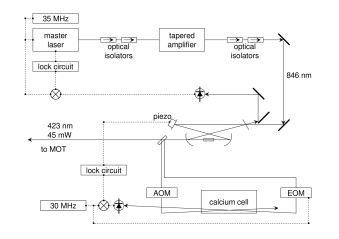
Figure 2: A schematic drawing of the MOT laser system and frequency stabilization electronics used in these experiments.

The laser is further stabilized by locking the 423 nm light to the calcium resonance transition using saturated absorption spectroscopy in a calcium vapor cell libbrecht95 . Our vapor cell differs from Ref. libbrecht95 in that it has a stainless steel body with conflat metal seals and windows and a valve. An acousto-optic modulator (AOM) in one arm of the saturated absorption laser beams shifts the laser frequency so that the laser beam sent to the MOT is 35 MHz (one natural linewidth) below the atomic resonance. We also use the AOM to chop this beam and use a lock-in amplifier to eliminate the Doppler background in the saturated absorption signal. Because the 846 nm laser is already locked to the frequency-doubling cavity, the feedback from this second lock circuit servos the frequency-doubling cavity length.

The trap is loaded from a thermal beam of calcium atoms that passes through the center of the MOT. The thermal beam is formed by heating calcium in a stainless steel oven to $650^{\mbox{\footnotesize{o}}}$ C. The beam is weakly collimated by a 1mm diameter, 10mm long aperture in the oven wall. The distance between the oven and the MOT is approximately 10 cm. As the beam passes through the MOT, the slowest atoms in the velocity distribution are cooled and trapped. An additional red-detuned (140 MHz, or four times the natural linewidth) laser beam counter-propagates the calcium atomic beam, significantly enhancing the MOT’s capture efficiency. To prevent optical pumping into metastable dark states we also employ a diode laser at 672 nm. The density profile of the MOT has an asymmetric Gaussian profile and is well-represented by Eq. 11 with the peak density equal to $4\times 10^{9}$ cm^-3, $\sigma_{0}=0.5$ mm, and $\alpha=2.5$.

We photo-ionize the atoms in the MOT using a two-color, two-photon ionization process. A portion of the 846 nm diode laser radiation from the MOT laser is pulse-amplified in a pair of YAG-pumped dye cells and frequency doubled. This produces a 3 ns-duration laser pulse at 423 nm with a pulse energy around 1 $\mu$J. This laser pulse passes through the MOT, and its peak intensity is a few thousand times greater than the saturation intensity. A second YAG-pumped dye laser at 390 nm counter-propagates the 423 nm pulse and excites the MOT atoms to low-energy states in the region of the ionization potential. We photo-ionize 85-90% of the ground-state atoms in the MOT. The minimum initial electron temperature is limited by the bandwidth of the 390 nm laser to about 1 K.

Ions in the plasma scatter light from a probe laser beam tuned to the Ca II ${}^{2}S_{1/2}-^{2}P_{1/2}$ transition at 397 nm. The probe laser is generated by a grating-stabilized violet diode laser. This laser, as well as the 672 nm laser used in the neutral atom trap, is locked to the calcium ion transition using the DAVLL technique corwin98 in a large-bore, low-pressure hollow cathode discharge of our own design (see Fig. 3).

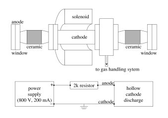
Figure 3: A schematic diagram of the DAVLL cell. Upper — A drawing of the hollow.cathode discharge cell, approximately to scale. The cathode is 10 cm long, with a 1 cm diameter bore. The operating pressure is between 100 and 200 mTorr of krypton. Lower — Electrical connections to the discharge cell. For increased current stability, a 2k$\Omega$ ballast resistor is connected in series with the discharge.

The probe laser is spatially filtered. The typical probe laser intensity is a few hundred $\mu$W focused to a Gaussian waist of 130 $\mu$m in the MOT. We average repeated measurements of the scattered 397 nm radiation with the probe laser in a given position, denoted by the parameter $a$ in Fig. 1. This produces a time-resolved signal proportional to the number of atoms resonant with the probe beam in a particular column of the plasma. By translating a mirror just outside the MOT chamber, we scan the probe laser across the ion cloud. In this manner we obtain temporal and spatial information about the plasma expansion.

IV Comparing the model to the data

One comparison of the isothermal model with experimental data was presented in Ref. cummings05 . In that work, the initial electron energy of the plasma, and therefore the expansion velocity $v_{e}$, was fixed, and the parameter $a$ was varied from 0 to 4$\sigma_{0}$.

In the following, we present a complementary comparison. The solid line in Fig. 4 shows ion fluorescence signal with the probe laser tuned to the ion resonance frequency, and with the probe laser beam propagating along the $z$ axis ($a=0$ in Fig. 1) for a range of initial electron energies.

As discussed in Ref. cummings05 , the early rise in the fluorescence signal shows the increasing number of plasma ions in the ${}^{2}P_{1/2}$ level. This feature is easily explained in terms of the classic Rabi two-level atom with damping. The probe laser intensity is in the range of 5 to 10 times the resonance Rabi frequency. Our numerical integration of the optical Bloch equations mimics the approximately 20 ns rise time observed in the experimental data, and shows that the Gaussian spatial profile of the probe laser beam washes out subsequent oscillations in the excited state fraction. Following the initial rise, the fluorescence decays. At approximately $t=50$ ns the decay slows down due to correlation-induced heating in the plasma simien04 ; cummings05 .

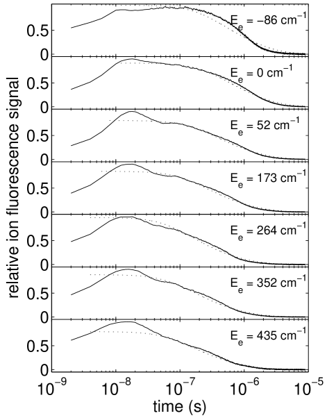
Figure 4: Relative ion fluorescence signal. The probe laser is tuned to resonance and propagates through the center of the plasma ($a=0$). The electron energy, $E_{e}$, is measured relative to the ionization limit. The solid line is the fluorescence signal, the dotted line is a fit using the Lorentzian lineshape in Eq. 18. The model is normalized to the fluorescence signal at $t=10^{-7}$ s, and the single fit parameter is the expansion velocity, $v_{e}$. In the top panel, the plasma is spontaneously generated after exciting the atoms to a Rydberg state with $n^{*}\sim 35.7$.

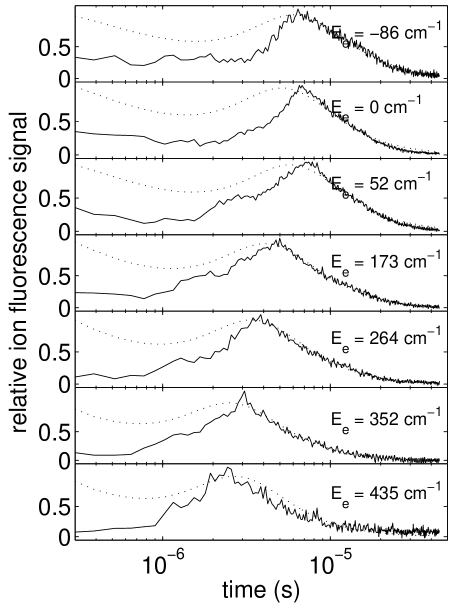
Figure 5: Relative ion fluorescence signal. The probe laser is tuned to resonance and propagates at a distance $a=1.1\mbox{mm}=2.2\sigma_{0}$ relative to the center of the initial distribution. The solid line is the data, and the dotted line is the fit using the Lorentzian lineshape in Eq. 18. The model is normalized to the peak of the data.

These two processes are not included in the isothermal model. We therefore begin the comparison of the model with the data at time $t=10^{-7}$ s. The model is normalized to the data and fit using $v_{e}$ as the only fit parameter in an un-weighted least-squares fitting routine. The model uses the Lorentzian lineshape in Eq. 18. The justification for using this lineshape arises from the analysis presented in Ref. cummings05 . In Fig. 2 of that reference, the $t=0$ velocity is 6 m/s. This is the rms velocity of a Boltzmann distribution, and it is due almost entirely to correlation-induced heating. This velocity width gives a Doppler width smaller than the natural line width, and the Voigt profile is close to a pure Lorentzian. Furthermore, as the plasma evolves, the ion temperature falls due to the adiabatic expansion. The time scale for this is $\sim\sigma_{0}/v_{e}=2\;\mu$s. This is shorter than the time scale for heating the ions by collisions with the electrons, $\sim m_{\mbox{\footnotesize{Ca}}}/m_{e}\omega_{p}=50\;\mu$s. It is therefore not surprising that the Gaussian lineshape gives a poorer fit to the data. In the fitting procedure, the Gaussian lineshape produces expansion velocities that do not grow as the initial electron energy increases. The figure shows that the Lorentzian model describes the data well over a few orders of magnitude in time. The velocities extracted from these data are shown in Fig. 6.

The differences between the model and the signal are not negligible. For all initial electron energies, the model is slightly too low at $t=300$ ns, and too high at $t>1\;\mu$s. The data are not corrected for optical pumping into the $D-$states, which we measure to have a time constant of about 5 $\mu$s. The differences between the model and the fluorescence signal could indicate internal heating processes that manifest themselves in the ion velocity on the few hundred ns time scale. They could also indicate ions that appear in the plasma from Rydberg states at late times or collective plasma density variations. These differences can be studied in future work.

We also compare the fluorescence signal and the model over a range of initial electron energies with the probe laser beam shifted to $a=1.1\mbox{mm}=2.2\sigma_{0}$. In this arrangement, the ion fluorescence signal is initially small, and grows as ions move into the probe laser beam. Typical data are shown in Fig. 5. For these data, the model is fit to the $t>6\;\mu$s signal using a least-squares procedure, with $v_{e}$ as the fit parameter. The velocity extracted from this fit is shown in Fig. 6. It is possible to fit the data using $v_{e}$ so that the peak in the model coincides with the peak of the fluorescence signal. These velocities are also plotted in the figure.

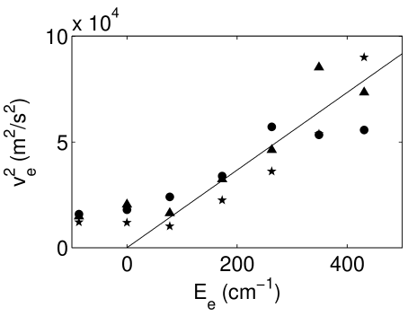
Figure 6: Expansion velocity extracted from Figs. 4 and 5. The triangles ($\blacktriangle$) represent the velocity extracted from Fig. 4, and the circles ($\bullet$) from Fig. 5. The stars ($\bigstar$) represent the velocity extracted from centering the peak of the model on the peak of the data in Fig. 5. The line is a fit of the data with $E_{e}>150$ cm^-1. The fitted result is $E_{e}=3.0mv_{e}^{2}$, where $m$ is the mass of the calcium ion.

.

For these data, the signal in the first $\mu$s is small compared to the model. Moreover, there are variations in the fluorescence signal that do not appear in the model. This suggests that at the edges of the plasma expansion, the density distribution is distinctly non-Gaussian, even at early times before any ion motion is possible. It also appears, as pointed out in Ref. cummings05 , that the Gaussian density profile is recovered at late times for all initial electron energies.

V conclusion

We present an extension of the isothermal plasma expansion model of Refs. robicheaux02 ; robicheaux03 for quasi-two-dimensional geometry. We include velocity effects and predict a fluorescence or absorption signal vs. time for given initial conditions. The model matches the correct order of magnitude and general features of the fluorescence signal. Some discrepancies are pointed out, which can be studied in future work.

Making the plasmas more ideally two-dimensional should improve applicability of the model, and further suppress effects due to expansion in the long dimension. Increasing the range of initial electron temperatures and plasma densities can probe interesting regions of phase space where differences between the data and the model are likely to be more pronounced.

As an example, it should be possible to extend this model to include effects due to electron-ion recombination at early times. For strongly-coupled neutral plasmas, the three-body recombination rate should be on the order of the plasma frequency. Using the high-sensitivity and fast time-response of fluorescence spectroscopy, it should be possible to directly measure spectroscopic recombination signatures in low-temperature, low-density plamsas, where the predicted three-body recombination rate is greater than the plasma frequency. For example, reducing the plasma density to 10⁶ cm^-3 will make the recombination time $\sim 1/\omega_{p}=20$ ns. Increasing the probe laser intensity to 100 times the saturation intensity will shorten the early rise time of the fluorescence signal to around 10 ns. Optical pumping time will be comparable to the correlation-induced heating time, around 200 ns.

VI Acknowledgements

This research is supported in part by Brigham Young University, the Research Corporation, and the National Science Foundation (Grant No. PHY-9985027). One of us (SDB) also acknowledges the support of the Alexander von Humboldt foundation.

References

- (1) T. C. Killian, S. Kulin, S. D. Bergeson, L. A. Orozco, C. Orzel, and S. L. Rolston Phys. Rev. Lett. 83, 4776 (1999)
- (2) S. Kulin, T. C. Killian, S. D. Bergeson, and S. L. Rolston Phys. Rev. Lett. 85, 318 (2000)
- (3) T. C. Killian, M. J. Lim, S. Kulin, R. Dumke, S. D. Bergeson, and S. L. Rolston Phys. Rev. Lett. 86, 3759 (2001)
- (4) C. E. Simien, Y. C. Chen, P. Gupta, S. Laha, Y. N. Martinez, P. G. Mickelson, S. B. Nagel, and T. C. Killian Phys. Rev. Lett. 92, 143001 (2004)
- (5) Y. C. Chen, C. E. Simien, S. Laha, P. Gupta, Y. N. Martinez, P. G. Mickelson, S. B. Nagel, and T. C. Killian Phys. Rev. Lett. 93, 265003 (2004)
- (6) E. A. Cummings, J. E. Daily, D. S. Durfee, and S. D. Bergeson arXiv:physics/0506069
- (7) S. D. Bergeson and R. L. Spencer Phys. Rev. E 67, 026414 (2003)
- (8) F. Robicheaux and James D. Hanson Phys. Rev. Lett. 88, 055002 (2002)
- (9) F. Robicheaux and James D. Hanson Phys. Plasmas 10, 2217 (2003)
- (10) S. G. Kuzmin and T. M. O’Neil, Phys. Rev. Lett. 88, 065003 (2002)
- (11) S. G. Kuzmin and T. M. O’Neil, Phys. Plasmas 9, 3743 (2002)
- (12) S. Mazevet, L. A. Collins, and J. D. Kress, Phys. Rev. Lett. 88, 055001 (2002).
- (13) T. Pohl, T. Pattard, and J. M. Rost, Phys. Rev. A 70, 033416 (2004)
- (14) T. Pohl, T. Pattard, and J. M. Rost, Phys. Rev. Lett. 94, 205003 (2005)
- (15) M. Bassetti and G. A. Erskine, CERN-ISR-TH/80-06
- (16) M. A. Furman, Am. J. Phys. 62, 1134 (1994)
- (17) Yuyan Liu, Jieli Lin, Guangming Huang, Yuanqing Guo, and Chuanxi Duan J. Opt. Soc. Am. B 18, 666 (2001)
- (18) M. L. Citron, H. R. Gray, C. W. Gabel, and C. R. Stroud, Jr. Phys. Rev. A 16, 1507 (1977)
- (19) E. L. Raab, M. Prentiss, Alex Cable, Steven Chu, and D. E. Pritchard Phys. Rev. Lett. 59, 2631 (1987)
- (20) A. D. Ludlow, H. M. Nelson, and S. D. Bergeson J. Opt. Soc. Am. B 18, 1813 (2001)
- (21) R. W. P. Drever, J. L. Hall, F. V. Kowalski, J. Hough, G. M. Ford, A. J. Munley, and H. Ward, Appl. Phys. B 31 97 (1983)
- (22) F. T.-Goudarzi and E. Riis, Opt. Commun. 227, 389 (2003)
- (23) Rodolphe Le Targat, Jean-Jacques Zondy, and Pierre Lemonde, arXiv:physics/0408031
- (24) K. G. Libbrecht, R. A. Boyd, P. A. Willems, T. L. Gustavson, and D. K. Kim, Am. J. Phys. 63, 729 (1995)
- (25) Kristan L. Corwin, Zheng-Tian Lu, Carter F. Hand, Ryan J. Epstein, Carl E. Wieman, Appl. Opt. 37, 3295 (1998)