On the origin of non-Gaussian statistics in hydrodynamic turbulence

Abstract

Turbulent flows are notoriously difficult to describe and understand based on first principles. One reason is that turbulence contains highly intermittent bursts of vorticity and strain-rate with highly non-Gaussian statistics. Quantitatively, intermittency is manifested in highly elongated tails in the probability density functions of the velocity increments between pairs of points. A long-standing open issue has been to predict the origins of intermittency and non-Gaussian statistics from the Navier-Stokes equations. Here we derive, from the Navier-Stokes equations, a simple nonlinear dynamical system for the Lagrangian evolution of longitudinal and transverse velocity increments. From this system we are able to show that the ubiquitous non-Gaussian tails in turbulence have their origin in the inherent self-amplification of longitudinal velocity increments, and cross amplification of the transverse velocity increments.

Intermittency in turbulent flows refers to the violent and extreme bursts of vorticity and rates of strain that occur interspersed within regions of relatively quiet flowFrisch95 . These infrequent, but extreme events are believed to cause observed deviations from the classical Kolmogorov theory of turbulenceKolmogorov41 . Intermittency also has a number of practical consequences since it can lead to sudden emergence of strong vortices in geophysical flowsSreeni99 , to modifications of the local propagation speed of turbulent flames Peters99 , etc. One of the observable manifestations of intermittency is the tendency of velocity increments, i.e. the difference between velocities at two spatial points separated by a distance $\ell$, to display highly non-Gaussian statistics when $\ell$ is smaller than the flow integral scale, $L$. The tails of velocity-increment probability density functions (pdf) are observed to be exponential and even stretched exponentialFrisch95 ; Sreeni99 . Moreover, an inherent asymmetry develops in the distribution of the longitudinal velocity increments, i.e. the difference of the velocity component in the direction of the displacement between the two points. This asymmetry yields the well-known negative skewness of longitudinal velocity incrementsFrisch95 . While the negativity of skewness can be derived from the Navier-Stokes (N-S) equations in isotropic turbulenceKolmogorov41 ; Frisch95 , a straightforward mechanistic explanation of the origins of stretched exponential tails, intermittency, and asymmetry has remained elusive.

In one dimension for the Burgers equation, the emergence of negative skewness and long negative tail in the pdf starting from random initial conditions is well understood based on the nonlinear term’s tendency to steepen the velocity gradient. In 3D turbulent flows, the notion of nonlinear “self-amplification” as the cause of intermittency has long been suspectedZeffetal03 . Yet, these expectations have eluded quantitative analysis due to the difficulty in deriving lower-dimensional models that maintain the relevant information about the vectorial nature of the full 3D dynamics. Many surrogate models have been proposed, such as shell models Biferale03 , the mapping closureKraichnan90 ; SheOrszag91 , etc, but the connection with the original N-S equations is typically based on qualitative and dimensional resemblances instead of on systematic derivation.

We consider the coarse-grained N-S equations filtered at scale $\Delta$ comparable (and larger) than the scale $\ell$. Let $\overline{u}_{i}$ be the filtered velocity field. Defining the velocity gradient tensor $\overline{A}_{ji}=\partial\overline{u}_{i}/\partial x_{j}$ and taking the gradient of the filtered N-S equations one obtainsVieillefosse84 ; Cantwell92 that the rate of change of the velocity gradient is given by

$$\dot{\overline{A}}_{ji}=-\left(\overline{A}_{jk}\overline{A}_{ki}+2Q/3~{}\delta_{ji}\right)+H_{ji},$$ (1)

where $Q=-\overline{A}_{mn}\overline{A}_{nm}/2$ arises from continuity. The tensor $H_{ji}$ contains the trace-free part of the pressure Hessian, subgrid, and viscous force gradientsBorueOrszag98 ; VanderBosetal02 : $H_{ji}=-(\partial^{2}_{ji}\overline{p}-\frac{1}{3}\delta_{ij}\partial^{2}_{kk}\overline{p})-(\partial^{2}_{jk}\tau_{ik}-\frac{1}{3}\delta_{ij}\partial^{2}_{lk}\tau_{lk})+\nu\partial^{2}_{kk}\overline{A}_{ji}$, in which $\overline{p}$ is the filtered pressure divided by density and $\nu$ the viscosity. $\tau_{ij}=\overline{u_{i}u}_{j}-\overline{u}_{i}\overline{u}_{j}$ is the subgrid-scale (SGS) stress. The time derivative $\dot{(\ )}$ is a Lagrangian material derivative defined as the rate of change of the gradient tensor following the local smoothed flow. Setting $H_{ij}=0$ yields the so-called “Restricted Euler” dynamicsVieillefosse84 ; Cantwell92 . A fruitful method to model the effects of $H_{ij}$ has been to track material deformations using either tetrad dynamicsChertkovetal99 or the Cauchy-Green tensorJeongGirimaji03 . Here we focus on a simpler object - a line element, aiming at identifying the mechanism generating intermittency. Thus, consider two points separated by a displacement vector $\bf r$ of length smaller than, or of the order of, $\Delta$ so that the local velocity field is smooth enough to be approximated as a linear field. The velocity increment between the two points over the displacement $\bf r$ is then

$$\delta u_{i}({\bf r},t)\equiv\overline{u}_{i}({\bf x}+{\bf r})-\overline{u}_{i}({\bf x})\approx\overline{A}_{ki}~{}r_{k}.$$ (2)

The longitudinal and transverse velocity increments, $\delta u(r,t)$ and $\delta v(r,t)$ respectively, can be evaluated from the two projections of velocity increment Eq. 2 into directions longitudinal and transverse to ${\bf r}$ (see FIG. 1):

$$\delta u(r,t)=\overline{A}_{ki}~{}r_{k}~{}\frac{r_{i}}{r},~{}~{}~{}~{}\delta v(r,t)=\left|P_{ij}({\bf r})\overline{A}_{kj}~{}r_{k}\right|,$$ (3)

where $P_{ij}({\bf r})=\delta_{ij}-r_{i}r_{j}/r^{2}$ and $r=|\bf r|$.

Note that $\delta u(r,t)$ and $\delta v(r,t)$ correspond to velocity increments over a displacement $r_{i}(t)$ that is evolving, in a local linear flow, according to equation $\dot{r}_{i}=\overline{A}_{mi}~{}r_{m}$. To study the evolution of velocity increments at a fixed scale $\ell$, it is necessary to eliminate effects from the changing distance between the two points. Consider a line that goes through the two points. Still within the assumption of a locally linear velocity field, the velocity increments across a fixed distance $\ell$ along this line are $\delta u\equiv\delta u(r,t){\ell}/{r}$, $\delta v\equiv\delta v(r,t){\ell}/{r}$ (see FIG. 1).

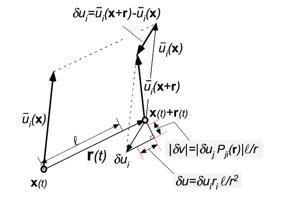
Figure 1: Illustrative sketch of velocity increment $\delta u_{i}({\bf r})$ between two points ${\bf x}(t)$ and ${\bf x}(t)+{\bf r}(t)$, and the components of $\delta u_{i}({\bf r})$ longitudinal and transverse to the displacement vector ${\bf r}$. The quantities of interest are $\delta u$ and $\delta v$, defined as the components of the velocity increment over a fixed length $\ell$.

Taking time derivatives of $\delta u$ and $\delta v$, and using the expressions for $\dot{\overline{A}}_{ji}$ and $\dot{r}_{i}$, many terms simplify and one arrives at the following “advected delta-vee” system of equations:

$$\delta\dot{u} = -{\delta u^{2}}~{}{\ell}^{-1}+{\delta v^{2}}~{}{\ell}^{-1}-\frac{2}{3}Q\ell+Y,$$ (4)

$$\delta\dot{v} = -{2~{}\delta u~{}\delta v}~{}{\ell}^{-1}+Z,$$ (5)

where $Y=\ell H_{ij}r_{i}r_{j}/r^{2}$ and $Z=\ell H_{ij}e_{j}r_{i}/r$ contain the anisotropic nonlocal effects of the pressure, inter-scale effects of subgrid-scale stresses, and damping effects of molecular viscosity (${\bf e}$ is a unit vector in the direction of the transverse velocity component). The first term on the right-hand-side (rhs) of the equation for $\delta\dot{u}$ also occurs in 1D Burgers equation (the self-amplification effect of negative velocity gradients). The second term indicates that the transverse velocity (rotation) tends to counteract the self-amplification process. For $\delta\dot{v}$, the first term on rhs of Eq. 5 suggests exponential growth of $\delta v$ at a rate $|\delta u|$ when $\delta u<0$. This “cross-amplification” mechanism can lead to very large values of $|\delta v|$.

We now pose the question whether the growth of intermittency and the asymmetry of longitudinal velocity increments can be understood based on this system of equations, but without the effects represented by $Y$ and $Z$ (i.e., “Restricted Euler” dynamics). In order to determine whether this simplified system approximates $\delta\dot{u}$ and $\delta\dot{v}$ in real turbulence, comparisons are made with direct numerical simulations (DNS). The rates of change of $\delta u$ and $\delta v$ predicted by DNS are obtained by finite difference in time from two DNS velocity fields separated by the simulation time-step $\delta t=0.001$. The data are obtained from a pseudo-spectral simulation of the N-S equations, with $256^{3}$ nodes and Taylor-scale Reynolds number $R_{\lambda}\approx 162$. The velocity fields are coarse-grained using a Gaussian filter of characteristic length $\Delta=40\eta$, where $\eta$ is the Kolmogorov length scale, yielding filtered velocity fields $\overline{u}_{i}({\bf x},t_{0})$ and $\overline{u}_{i}({\bf x},t_{0}+\delta t)$ ($i=1,2,3$). At the initial time $t_{0}$, to every grid-point ${\bf x}(t_{0})$ on the computational mesh, we associate a partner ${\bf x}(t_{0})+{\bf r}(t_{0})$ at a distance $|{\bf r}(t_{0})|=\ell=40\eta$ in some Cartesian direction. For each pair of points we measure the longitudinal and transverse velocity increments. Then, we find the position to which ${\bf x}(t_{0})$ and ${\bf x}(t_{0})+{\bf r}(t_{0})$ will be advected by the smoothed velocity field, which are, using simple Euler integration, ${\bf x}(t_{0}+\delta t)={\bf x}(t_{0})+\overline{\bf u}({\bf x},t_{0})\delta t$, and ${\bf x}(t_{0}+\delta t)+{\bf r}(t_{0}+\delta t)$, where ${\bf r}(t_{0}+\delta t)={\bf r}(t_{0})+[\overline{\bf u}({\bf x}(t_{0})+{\bf r}(t_{0}),t_{0})-\overline{\bf u}({\bf x}(t_{0}),t_{0})]\delta t$ is the new displacement vector. The final end-point at a fixed distance $\ell$ is found by moving the material end-point ${\bf x}(t_{0}+\delta t)+{\bf r}(t_{0}+\delta t)$ along the new displacement vector to the point ${\bf x}(t_{0}+\delta t)+{\bf r}(t_{0}+\delta t)\ell/|{\bf r}(t_{0}+\delta t)|$, so that the distance is kept fixed. Velocities at the new locations are obtained from the stored field at the new time using bilinear interpolation, and the longitudinal and transverse components are evaluated, by projections onto direction parallel and perpendicular to the new displacement vector between the two points. The rate of change of $\delta u$ and $\delta v$ is evaluated using first-order finite difference in time. Conversely, the rates of change predicted by the model system are evaluated as $-\delta u^{2}/\ell+\delta v^{2}/\ell-(2/3)Q\ell$ and $-2~{}\delta u~{}\delta v/\ell$ from the measured values of $\delta u$, $\delta v$ and $Q$. Both real and modeled rates of change are computed over a large number of points in the DNS data, and their correlation coefficient and joint pdf are evaluated.

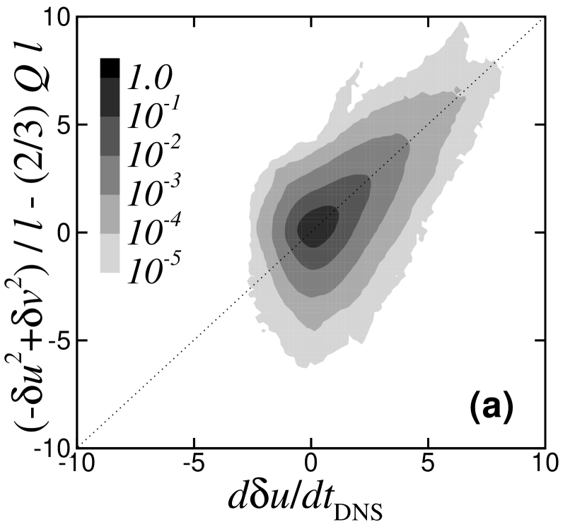
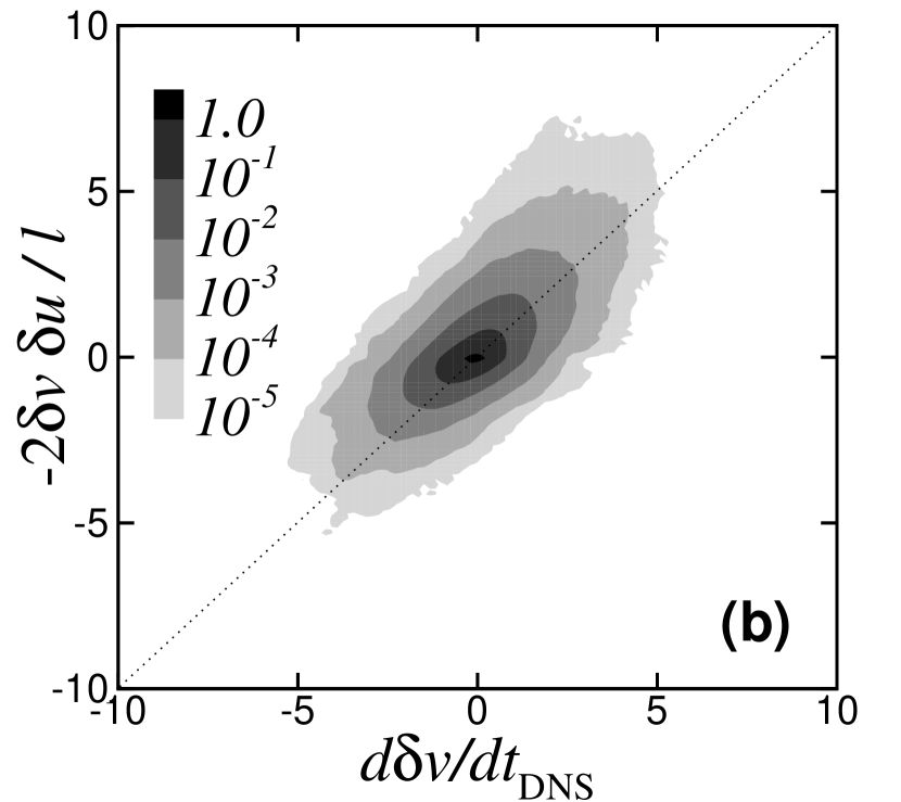
Figure 2: Joint pdf of rates of change of velocity increments predicted from DNS (filtered at $\Delta=40\eta$ and taking increments over a distance $\ell=40\eta$) and the “advected delta-vee” system. (a) longitudinal and (b) transverse velocity increments. Results are robust with changes in $\Delta$ and $\ell$ (with $\ell\leq\Delta$).

FIG. 2 shows the joint pdf of the model results versus the rates of change measured from DNS. A clear correlation can be seen between model and DNS results. Correlation coefficients are $0.54$ for the longitudinal and $0.61$ for the transverse velocity increments, indicating that the model system captures important (but clearly not all) effects seen in the real dynamics. The deviations between model system and DNS are caused by the neglected $Y$ and $Z$ terms, to be studied in future work.

After confirming that the simplified system captures important trends in 3D fluid turbulence, we explore the trends predicted by solutions of the model system. In the present Letter we set $Q$ to a constant $Q_{0}$ (numerical tests show that allowing $Q$ to evolve in time leads to the same short-time behavior to be displayed below, except if $Q$ were to be closely correlated with $\delta u$ and $\delta v$, which is not the case in 3D turbulence, since $Q$ depends on velocity gradients along two additional directions.). We note that for $Q=0$, the system describes the relative motion of a fluid (with a locally linear velocity field) consisting of non-interacting (“ballistic”) particles that maintain their initial velocity. For $Q\neq 0$, the particles are subjected to a relative force equal to the spherical average of the pressure, inter-scale, and viscous damping forces. For the case $Q_{0}=0$ the analytical solution is

$$\delta u(t)=\ell e_{0}[e_{0}t+\delta u_{0}\ell]/\{[e_{0}t+\delta u_{0}\ell]^{2}+\delta v_{0}^{2}\ell^{2}\},$$ (6)

$$\delta v(t)=\ell^{2}\delta v_{0}e_{0}/\{[e_{0}t+\delta u_{0}\ell]^{2}+\delta v_{0}^{2}\ell^{2}\},$$ (7)

where $e_{0}=\delta u_{0}^{2}+\delta v_{0}^{2}$. For discrete values of time, this defines a mapping (the “advected delta-vee map”). The system has an invariant

$$U_{0}=(\delta u^{2}+\delta v^{2})/\delta v,$$ (8)

and its (circular) phase-space trajectories are $\delta u^{2}+(\delta v-U_{0}/2)^{2}=(U_{0}/2)^{2}$, as shown in FIG. 3.

Figure 3: Phase-space portrait of the “advected delta-vee” dynamical system ${\delta\dot{u}}=-\delta u^{2}+\delta v^{2}$, $\delta\dot{v}=-2~{}\delta u~{}\delta v$ (for $Q_{0}=0$ and $\ell=1$).

In order to illustrate the evolution of $\delta u(t)$ and $\delta v(t)$, we start from an ensemble of randomly oriented lines for which the velocity increment vectors are initialized from a Gaussian distribution. The increments $\delta u(t)$ and $\delta v(t)$ over these lines are evaluated at several later times. To compare with experimental data, two issues need to be considered. First, since $\delta v(t)$ is the magnitude of the transverse velocity increment vector, it has to be projected onto a coordinate direction to obtain a component of the transverse increment, $\delta v_{c}=\delta v\cos\theta$. For isotropic turbulence, the angle $\theta$ between the vector and a fixed direction in the transverse plane is uniformly distributed in $[0,2\pi)$. Therefore, the pdf $P^{c}_{v}(\delta v_{c})$ of $\delta v_{c}$ is related to that of $\delta v$, $P_{v}(\delta v)$, by

$$P^{c}_{v}(\delta v_{c})=\frac{1}{\pi}\int_{|\delta v_{c}|}^{+\infty}P_{v}(\delta v)\frac{d\delta v}{\sqrt{\delta v^{2}-\delta v^{2}_{c}}}.$$ (9)

Second, an ensemble of randomly oriented lines (with uniform measure on a sphere, i.e. a uniform distribution of initial solid angles $d\Omega_{0}$) will tend to concentrate along directions of positive elongation. Thus, in order to compare model results at later times with data that are taken at random directions not correlated with the dynamics, the model results need to be weighted with the evolving solid angle measure. Conservation of fluid volume implies that $\ell^{3}d\Omega_{0}=r(t)^{3}d\Omega(t)$, i.e. in directions of growing $r(t)$, the solid angle $d\Omega(t)$ decreases. Thus, probabilities must be weighted by

$$d\Omega(t)/d\Omega_{0}=[\ell/r(t)]^{3}.$$ (10)

Since $\dot{r}=\delta u\,r/\ell$, we can solve for $r(t)$ and then obtain $d\Omega(t)/d\Omega_{0}=\exp(-3\ell^{-1}\int_{0}^{t}\delta u(t^{\prime})dt^{\prime})$. Using the solution for $\delta u$, we obtain $d\Omega(t)/d\Omega_{0}=\ell^{3}[(\ell+\delta u_{0}t)^{2}+\delta v_{0}^{2}t^{2}]^{-3/2}$ for $Q_{0}=0$. This factor is used to weight the measured time-evolving pdfs from the model system. Note that when $\delta v_{0}\to 0$ and $\delta u_{0}<0$, there is an unphysical finite time singularity at $t\to\ell/|\delta u_{0}|$, when $r\to 0$.

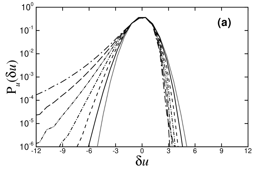
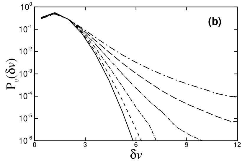
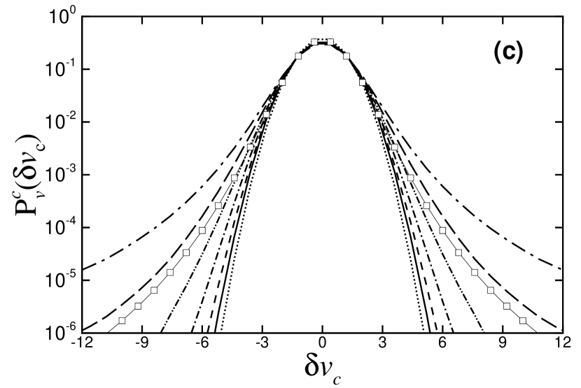
Figure 4: Evolution of the pdf of velocity increments in time: (a) longitudinal velocity increment, (b) the magnitude and (c) a component of the transverse velocity increment vector. $\delta u$ is initialized as a standard Gaussian random number and $\delta v$ as the square root of the sum of the square of two independent Gaussian random numbers. (c) is calculated from (b) by numerical integration of Eq. (9). For simplicity, we set $\ell=1$, so that the characteristic time-scale of the ensemble is $\tau=\ell/\delta u_{0}|_{\rm rms}=1$. Dotted line in (a) and (c): Gaussian; solid: $t=0.03$; dashed: $t=0.06$; dash-dotted: $t=0.09$; dash-double-dotted: $t=0.12$; long-dashed: $t=0.15$; long-dash-dotted: $t=0.18$; and thin line with squares in (c): $t=0.18$ without correcting for evolving measure.

FIG. 4 shows the evolution of the pdfs of the longitudinal and transverse velocity increments (both the magnitude and a component), as time progresses (for the case $Q_{0}=0$). It is immediately clear that the two main qualitative trends observed in turbulence naturally evolve from the solution of the system: the skewness towards negative values of longitudinal velocity increment, and the noticeable flare-up of long tails in the pdfs of transverse velocity increment. Also, these features appear rather quickly: after a non-dimensional time $t/\tau=0.18$ the pdf is already highly skewed and displays stretched exponential tails. Very similar results are observed for nonzero values of $Q_{0}$ (using numerical forward time integration with a standard fourth order Runge-Kutta routine, we tested $Q_{0}=\pm 2$): Relative to the results for $Q_{0}=0$, the pdfs of $\delta u$ are shifted to the left for $Q_{0}>0$ and to the right for $Q_{0}<0$, and only very minor differences are seen for $\delta v$. The rapid appearance of stretched exponential tails is due to the divergence of the phase-space trajectories on the left half of the plane in FIG. 3. For a given initial kinetic energy $\delta u_{0}^{2}+\delta v_{0}^{2}$, if $\delta v_{0}$ is small, the invariant $U_{0}$ can be arbitrarily large. Thus $\delta u$ and $\delta v$ can later grow to very large values during the evolution.

In summary, the model system proves useful in showing that the emergence of ubiquitous trends of 3D turbulence, namely intermittent and asymmetric tails in pdfs of velocity increments, occur even in the “ballistic” case ($Q_{0}=0$). Considering all possible random initial directions of relative motion, the fraction of particle pairs that initially move towards each other is small, thus large gradients in small spatial regions occur rather infrequently but are very intense when they occur due to the self-amplification mechanism for $\delta u$, and the cross-amplification mechanism for $\delta v$. While the model system thus helps explain the origin and trends towards intermittency in 3D turbulence, predicting quantitatively the level of intermittency remains an open question. It requires understanding the effects of pressure, inter-scale interactions (that depends on interactions of vorticity and strains at various scales, see e.g. Abidetal02 ; Taoetal02 ) and viscosity that are neglected in the model system. But already, the proposed model system could be combined with cascade, mapping closure, or shell models to enable these heuristic approaches to include a more direct link to the underlying Navier-Stokes equations.

- (1) U. Frisch, Turbulence: the legacy of A. N. Kolmogorov (Cambridge university press, Cambridge, 1995).
- (2) A. N. Kolmogorov, Dokl. Akad. Nauk. SSSR 30, 301 (1941); reprinted in Proc. R. Soc. Lond. A 434, 9 (1991).
- (3) K. R. Sreenivasan, Rev. Mod. Phys. 71, S383 (1999).
- (4) N. Peters, J. Fluid Mech. 384, 107 (1999).
- (5) B. W. Zeff et al., Nature 421, 146 (2003).
- (6) L. Biferale, Annu. Rev. Fluid Mech. 35, 441 (2003).
- (7) R. H. Kraichnan, Phys. Rev. Lett. 65, 575 (1990).
- (8) Z.-S. She and S. A. Orszag, Phys. Rev. Lett. 66, 1701 (1991).
- (9) P. Vieillefosse, Physica A 125, 150 (1984).
- (10) B. J. Cantwell, Phys. Fluids A 4, 782 (1992).
- (11) V. Borue and S. A. Orszag, J. Fluid Mech. 366, 1 (1998).
- (12) F. van der Bos, B. Tao, C. Meneveau, and J. Katz, Phys. Fluids 14, 2456 (2002).
- (13) M. Chertkov, A. Pumir, and B. I. Shraiman, Phys. Fluids 11, 2394 (1999).
- (14) E. Jeong and S. S. Girimaji, Theoret. Comput. Fluid Dynamics 16, 421 (2003).
- (15) M. Abid, B. Andreotti, S. Douady, and C. Nore, J. Fluid Mech. 450, 207 (2002).
- (16) B. Tao, J. Katz, and C. Meneveau, J. Fluid Mech. 457, 35 (2002).