Wave scattering by metamaterial wedges and interfaces

Abstract

We outline specific features of numerical simulations of metamaterial wedges and interfaces. We study the effect of different positioning of a grid in the Yee method, which is necessary to obtain consistent convergence in modeling of interfaces with metamaterials characterized by negative dielectric permittivity and negative magnetic permeability. We demonstrate however that, in the framework of the continuous-medium approximation, wave scattering on the wedge may result in a resonant excitation of surface waves with infinitely large spatial frequencies, leading to non-convergence of the simulation results that depend on the discretization step.

16002800

A.A. Sukhorukov, I.V. Shadrivov, and Yu.S. KivsharWave scattering by metamaterial wedges and interfaces

ans124@rsphysse.anu.edu.au

1 INTRODUCTION

Recent theoretical [1, 2, 3, 4] and experimental [5, 6, 7] studies have shown the possibility of creating novel types of microstructured materials that demonstrate the property of negative refraction. In particular, the composite materials created by arrays of wires and split-ring resonators were shown to possess both negative real parts of magnetic permeability and dielectric permittivity for microwaves. These materials are often referred to as left-handed metamaterials, double-negative materials, negative-index materials, or materials with negative refraction. Properties of such materials were first analyzed theoretically by V. Veselago a long time ago [8], but they were demonstrated experimentally only recently. As was shown by Veselago [8], left-handed metamaterials possess a number of peculiar properties, including negative refraction for interface scattering, inverse light pressure, reverse Doppler effect, etc.

Many suggested and demonstrated applications of negative-index metamaterials utilize unusual features of wave propagation and scattering at the interfaces. In particular, the effect of negative refraction can be used to realize focusing with a flat slab, the so-called planar lens [8]; in a sharp contrast with the well-known properties of conventional lenses with a positive refractive index where curved surfaces are needed to form an image. Moreover, the resolution of the negative-index flat lens can be better than a wavelength due to the effect of amplification of evanescent modes [9].

Direct numerical simulations provide the unique means for a design of microwave and optical devices based on the negative-index materials, however any realistic simulation should take into account metamaterial dispersion and losses [10, 11, 12, 13] as well as a nonlinear response [14]. Such numerical simulations are often carried out within the framework of the effective medium approximation, when the metamaterial is characterized by the effective dielectric permittivity and magnetic permeability. This simplification allows for modelling of large-scale wave dynamics using the well-known finite-difference time-domain (FDTD) numerical methods [15].

In this paper, we discuss the main features and major difficulties in applying the standard FDTD numerical schemes for simulating wave scattering by wedges and interfaces of finite-extend negative-index metamaterials, including a key issue of positioning of a discretization grid in the numerical Yee scheme [16] necessary to obtain consistent convergence in modeling surface waves at an interface between conventional dielectric and metamaterial with negative dielectric permittivity and negative magnetic permeability. In particular, we demonstrate that, in the framework of the continuous-medium approximation, wave scattering on the wedge may result in a resonant excitation of surface waves with infinitely large spatial frequencies, leading to non-convergence of the simulation results that depend on the discretization step.

2 BASIC EQUATIONS

We consider a two-dimensional problem for the propagation of TE-polarized electromagnetic waves in the plane $(x,z$), where the medium properties are isotropic and characterized by the dielectric permittivity $\varepsilon$ and magnetic permeability $\mu$. In the absence of losses, ${\cal I}m\;\varepsilon={\rm Im}\;\mu=0$. The response of negative-index materials is known to be strongly frequency dependent [1], however in the linear regime the wave propagation at different wavelengths can be described independently. The stationary form of Maxwell’s equation for the complex wave envelopes is well-known

$$\frac{\partial H_{z}}{\partial x}-\frac{\partial H_{x}}{\partial z}=\frac{i\omega}{c}\varepsilon(x,z)E_{y},\quad\frac{\partial E_{y}}{\partial z}=-\frac{i\omega}{c}\mu(x,z)H_{x},\quad\frac{\partial E_{y}}{\partial x}=\frac{i\omega}{c}\mu(x,z)H_{z},$$ (1)

where $H_{x}$, $H_{z}$, and $E_{y}$ are the components of the magnetic and electric fields, respectively, $\omega$ is angular frequency, and $c$ is the speed of light in vacuum. The system of coupled equations (1) can be reduced to a single Helmholtz-type equation for the electric field envelope,

$$\mu(x,z)\frac{\partial}{\partial x}\left(\frac{1}{\mu(x,z)}\frac{\partial E_{y}}{\partial x}\right)+\mu(x,z)\frac{\partial}{\partial z}\left(\frac{1}{\mu(x,z)}\frac{\partial E_{y}}{\partial z}\right)+\frac{\omega^{2}}{c^{2}}n^{2}(x,z)E_{y}=0,$$ (2)

where $n^{2}(x,z)=\epsilon(x,z)\mu(x,z)$, and $n$ is the refractive index of the medium.

3 WAVE SCATTERING BY A NEGATIVE-INDEX SLAB

The concept of perfect sub-wavelength imaging of a point source through reconstitution of the evanescent waves by a flat lens has remained highly controversial [17] because it is severely constrained by anisotropy and losses of the metamaterials. Nevertheless, several numerical studies showed that nearly-perfect imaging should be expected even under realistic conditions when both dispersion and losses are taken into account [10, 11, 12, 13]. In this section, we consider the numerical simulations of the wave scattering by a slab of the negative-index material, i.e. the problem close to that of the perfect lens imaging, and discuss the convergence of the Yee numerical discretization scheme.

3.1 Geometry and discretization

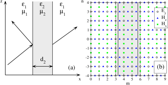
Figure 1: (a) Geometry of the scattering problem, the slab of the thickness $d_{2}$ is made of a negative-index metamaterial with both $\epsilon_{2}$ and $\mu_{2}$ negative. (b) Discretization scheme in the Yee method.

We start our analysis by considering wave propagation through a slab made of the negative-index material, as schematically illustrated in Fig. 1, with homogeneous properties in the $(y,z)$ plane characterized by two functions, the electric permittivity $\varepsilon=\varepsilon(x)$ and magnetic permeability $\mu=\mu(x)$. To solve this problem numerically, we employ the well-known numerical Yee method [15] and perform the discretization of the electric and magnetic fields on a square grid ($x_{m}=h\;m$, $z_{n}=h\;n$) presenting the fields in the form,

$$E_{y}|_{m,n}=\langle E_{y}\rangle_{m,n},\quad H_{z}|_{m+1/2,n}=\langle H_{z}\rangle|_{m+1/2,n},\quad H_{x}|_{m,n+1/2}=\langle H_{x}\rangle|_{m,n+1/2},\quad$$ (3)

where we use the notation

$$\langle\bullet\rangle_{n,m}=\int_{x_{m-1/2}}^{x_{m+1/2}}\int_{z_{n-1/2}}^{z_{n+1/2}}\bullet\;dx\;dz.$$

Then, we replace the continuum model by a closed set of the discrete equations for the field amplitudes obtained by averaging equations (1) over the cells of discretization mesh, taking into account the continuity of the tangential field components at the interface [15],

$$\begin{array}[]{l}{\displaystyle\frac{H_{z}|_{m+1/2,n}-H_{z}|_{m-1/2,n}}{h}-\frac{H_{x}|_{m,n+1/2}-H_{x}|_{m,n-1/2}}{h}=\frac{i\omega}{c}\left\langle\varepsilon\right\rangle_{m,n}E_{y}|_{m,n},}\\[12.0pt] {\displaystyle\frac{E_{y}|_{m,n+1}-E_{y}|_{m,n}}{h}\langle{\mu^{-1}}\rangle_{m,n+1/2}=-\frac{i\omega}{c}H_{x}|_{m,n+1/2},}\\[12.0pt] {\displaystyle\frac{E_{y}|_{m,n}-E_{y}|_{m+1,n}}{h}=\frac{i\omega}{c}\left\langle\mu\right\rangle_{m+1/2,n}H_{z}|_{m+1/2,n}.}\end{array}$$ (4)

Whereas the general form of the discrete equations (4) is well known [15], we point out a number of specific features arising in numerical simulations of the waves scattering at the interfaces with the negative-index media. Since the real parts of both $\varepsilon$ and $\mu$ change sign at these interfaces, the corresponding averaged values may become small or even vanish for a certain layer position with respect to the numerical grid. In this case, Eqs. (4) may become (almost) singular, leading to poor convergence. In this paper, we suggest that consistent convergence can be achieved by artificially shifting the layer boundary with respect to the grid in order to ensure that the averaged values do not vanish. This shift will not exceed $h/2$, assuring convergence as the step-size is decreased.

Because the tangential component $E_{y}$ of the electric field should be continuous at the interface, is seems that a natural choice is to align the boundary position with the grid points $x_{m}$, where $E_{y}|_{m,n}$ is defined, and we use this configuration in the numerical simulations presented below. However, we note that such a selection leads to singularities for averaged values if $\varepsilon_{1}=-\varepsilon_{2}$ or $\mu_{1}=-\mu_{2}$, which coincides with the flat-lens condition. Therefore, it is necessary to take into account losses in the metamaterial, described by nonzero imaginary parts of the complex values $\varepsilon_{2}$ and $\mu_{2}$, or to choose a different boundary alignment to the grid for the numerical simulations of perfect lenses [1].

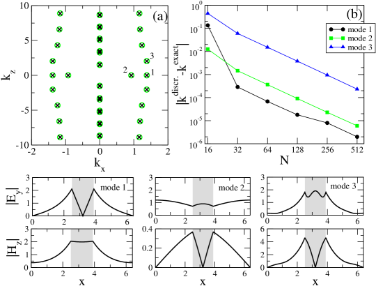
Figure 2: (a) Spectrum of wavenumbers $k_{z}$ for a negative-index layer: exact (circles) and discrete (crosses, for $N=512$) solutions. (b) Absolute differences between the exact and discrete values of $k_{z}$ vs. the number of points ($N$) along $x$ for the marked points 1,2,3 in (a). Bottom: Mode profiles marked 1,2,3 in (a). The computational domain is $0<x<6.4$, $d_{2}=1.4$ is the width of the negative-index layer with $\varepsilon_{2}=-1.2$ and $\mu_{2}=-1.5$, and $\varepsilon_{1}=\mu_{1}=1$. The wavenumber in vacuum is normalized as $\omega/c=1$.

3.2 Wave spectrum and convergence of discrete solutions

In order to illustrate the convergence of the proposed numerical scheme, we compare the solutions of discrete and continuous equations. We note that wave scattering from an infinite layer is fully characterized by the properties of spatial modes, which wavevector components along the layer ($k_{z}$) are conserved. These modes have the form

$${\bf E}(x,z)={\cal E}(x;\;k_{z}){\rm exp}(ik_{z}z),\quad{\bf H}(x,z)={\cal H}(x;\;k_{z}){\rm exp}(ik_{z}z).$$ (5)

Substituting Eqs. (5) into Eq. (1) and Eq. (4), we obtain a set of corresponding continuous and discrete eigenmode equations. For every $k_{z}$, the mode profiles can be determined analytically, e.g., using the transfer-matrix method [18]. The wave spectrum can contain solutions corresponding to the guided modes of a negative-index layer [19], and extended (or propagating) modes that should also be taken into account as well, in order to describe scattering of arbitrary fields.

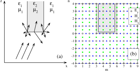
Figure 3: (a) Geometry of the scattering problem, the finite-extent slab is made of a negative-index metamaterials with both $\epsilon_{2}$ and $\mu_{2}$ negative. (b) Discretization scheme in the Yee method.

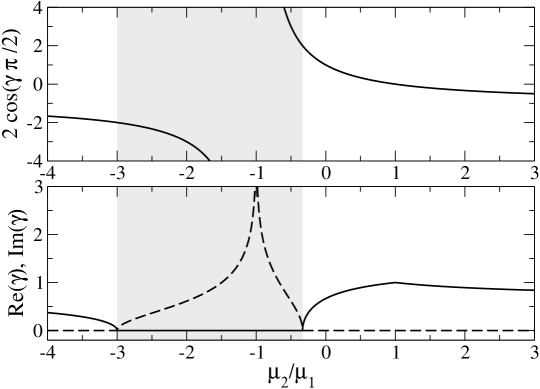
Figure 4: Dependence of (a) the cosine of the singularity parameter and (b) its real (solid) and imaginary (dashed) parts on $\mu_{2}/\mu_{1}$ according to Eq. (6). Shading marks the region with ${\cal I}m\gamma\neq 0$.

We solve the discrete eigenmode equations numerically for the slab geometry with periodic boundary conditions, and compare the spectrum of eigenvalues $k_{z}$ with exact solutions of the continuous model. In Fig. 2(a), we show a part of the spectrum of the discrete eigenvalues (crosses), which indeed coincides with the exact values (circles). The rate of convergence can be judged from Fig. 2(b), where the differences between the approximate and exact solutions are shown in logarithmic scale.

4 WAVE SCATTERING BY A WEDGE OF NEGATIVE-INDEX MATERIAL

One of the fundamental problems in the theory of negative-index metamaterials is the wave scattering by wedges [20], where convergence of numerical methods can be slow due to the appearance of singularities [21]. In this section, we demonstrate that the nature of such singularities has to be taken into account when performing FDTD numerical simulations.

4.1 Singularity parameter

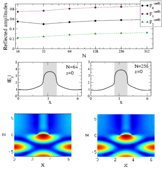
Figure 5: (a) Amplitudes of reflected plane waves vs. the number of points; (b,c) Electric field profiles for $N=64$ and $N=256$. Parameters are the same as in Fig. 2, except $\mu_{2}=-3.5$.

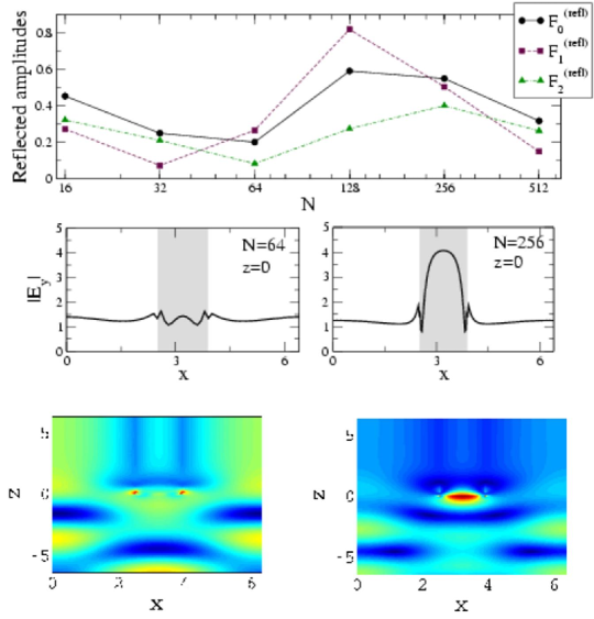
Figure 6: (a) Amplitudes of reflected plane waves vs. the number of points; (b,c) Electric field profiles for $N=64$ and $N=256$. Parameters are the same as in Fig. 2.

The behavior of the electric and magnetic fields at the wedges between homogeneous materials characterized by different values of $\varepsilon$ and $\mu$ was described analytically in the pioneering paper of Meixner [21] and further refined in the subsequent studies (see, e.g., Ref. [22], and references therein). In the case of the TE wave scattering by a negative-index wedge, as schematically illustrated in Fig. 3, the amplitudes of magnetic fields exhibit singular behavior at the wedge of the order of $\rho^{\gamma-1}$, where $\rho$ is the distance from the wedge. For a $\pi/2$ wedge angle, corresponding to a corner of a rectangular slab, the coefficient $\gamma$ is found as [21]

$$\frac{\mu_{1}-\mu_{2}}{\mu_{1}+\mu_{2}}=\pm 2{\rm cos}\left(\gamma\pi/2\right),$$ (6)

where $\mu_{1}$ and $\mu_{2}$ are magnetic permeabilities of the two neighboring media. In the case of conventional dielectric or magnetic media with $\mu_{j}>0$, Eq. (6) has solutions with real $\gamma$. However, when $\mu$ changes its sign at the interface with a negative-index medium, the coefficient $\gamma$ becomes complex playing role of a singularity parameter. This happens when

$$-3\mu_{1}<\mu_{2}<-\mu_{1}/3,$$ (7)

so that $|\mu_{1}-\mu_{2}|/|\mu_{1}+\mu_{2}|>2$, see Fig. 4.

For real $\gamma$ (taking the solution with $0<\gamma<1$, according to Ref. [21]), the field amplitudes decay monotonously away from the corner. In this case, numerical simulations may be based on the simplest discretization, although the convergence rate can be improved by taking into account the singular behavior in the discrete equations.

However, the case of complex $\gamma$ corresponds to the fields that oscillate infinitely fast near the corner because

$$\rho^{\gamma-1}=\rho^{{\cal R}e(\gamma-1)}\exp\left[i\,{\cal I}m(\gamma)\,\log(\rho)\right].$$

The second multiplier indicates the excitation of infinitely large spatial harmonics, however such a situation is unphysical because the effective-medium approximation of the negative-index materials is valid for slowly varying fields only. Therefore, in numerical simulations it is necessary to take into account the physical effects that suppress such oscillations, in particular we discuss the effect of losses in Sec. 4.3 below.

4.2 Numerical results

We now analyze convergence of the numerical finite-difference solutions for the problem of wave scattering by a finite-extent negative-index slab. We align the boundaries of the negative-index domain with the grid, as shown schematically in Fig. 1(b). Since the electric field components $E_{y}$ are continuous at the interfaces, it is possible to obtain the discrete equations that have the form of Eqs. (4).

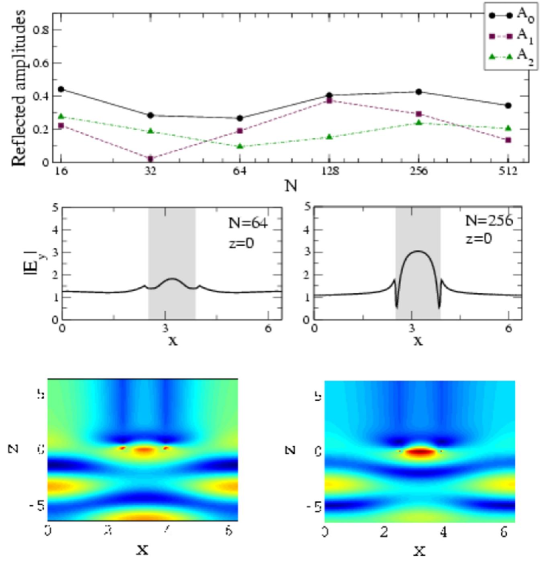
Figure 7: Same as in Fig. 6 but for $\mu=-1.5+i\;10^{-1}$.

In order to construct the full solutions for scattering problem, we decompose the field into a set of eigenmodes of the negative-index layer ($z>0$) and free space ($z<0$). More specifically, for $z>0$ we have

$${\bf E|_{m,n}}=\sum_{j}A_{j}{\cal E}|_{m,n}(k_{z}^{(j)}){\rm exp}(ik_{z}^{(j)}z_{n}),\quad{\bf H|_{m,n}}=\sum_{j}A_{j}{\cal H}|_{m,n}(k_{z}^{(j)}){\rm exp}(ik_{z}^{(j)}z_{n}),$$ (8)

where $j$ is the number of eigenmodes. Here the summation is performed over the propagating modes (${\cal I}mk_{z}=0$) which transport energy away from the interface, and evanescently decaying modes with ${\cal I}mk_{z}<0$. In free space at $z<0$, the field is composed of incident and reflected plane waves,

$$E_{y}|_{m,n}=\sum_{j=-N/2+1}^{N/2}F_{j}^{\rm(in)}\exp(i2\pi jm/N+iK^{(j)}z_{n})+\sum_{j=-N/2+1}^{N/2}F_{j}^{\rm(refl)}\exp(i2\pi jm/N-iK^{(j)}z_{n}).$$ (9)

Here $N$ is the number of points in the $x$ direction, and the discrete wavenumber is $K^{(j)}=\pm{\rm sin}^{-1}\left[h^{2}\omega^{2}/4c^{2}-{\rm sin}^{2}(j\pi/N)\right]^{1/2}2/h$ [15]. The sign of $K^{(j)}$ is chosen with a proper wave asymptotic behavior, i.e., we choose ${\cal R}e(K^{(j)})>0$, if $K^{(j)}$ is real, and ${\cal I}m(K^{(j)})>0$ if $K^{(j)}$ is complex. The magnetic field at $z<0$ is found from Eq. (4), with homogeneous parameters $\langle\varepsilon\rangle=\varepsilon_{1}$, $\langle\mu\rangle=\mu_{1}$, $\langle\mu^{-1}\rangle=\mu_{1}^{-1}$. Then, we substitute Eqs. (8), (9) into the first of Eq. (4), and using the condition of the continuity of the electric field, obtain a set of equations for all $m=1,\ldots,N$ that are used to calculate the amplitudes $F_{j}^{(refl)}$ and $A_{j}$ of the reflected and transmitted waves,

$$\begin{array}[]{l}{\displaystyle\sum_{j}A_{j}{\cal E}_{y}|_{m,0}(k_{z}^{(j)})=\sum_{j=-N/2+1}^{N/2}(F_{j}^{\rm(in)}+F_{j}^{\rm(refl)})\exp(i2\pi jm/N)}\\[12.0pt] {\displaystyle\sum_{j}A_{j}\left[{\cal H}_{x}|_{m,-1/2}(k_{z}^{(j)})+{\cal H}_{x}|_{m,1/2}(k_{z}^{(j)})\right]}\\[12.0pt] {\displaystyle\qquad=\frac{-2c}{\omega\mu_{1}h}\sum_{j=-N/2+1}^{N/2}(F_{j}^{\rm(in)}-F_{j}^{\rm(refl)})\sin(K^{(j)}h)\exp(i2\pi jm/N).}\end{array}$$ (10)

These equations are solved using the standard linear algebra package.

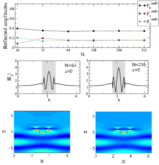
Figure 8: Same as in Fig. 6 but for $\mu=-1.01+i\;10^{-2}$.

We now present results of our numerical simulations for the scattering of normally incident plane waves, with $F_{0}^{(in)}=1$, $F_{j\neq 0}^{(in)}=0$. First, we consider scattering by a negative-index slab with $\mu_{2}<-3$. In this case, we observe a steady convergence of numerical solutions, as shown in Fig. 5. This demonstrates that even simplest finite-difference numerical schemes can be successfully employed to model the scattering process when the sinularity parameter $\gamma$ is real, is in a full agreement with earlier studies of wave scattering at dielectric wedges [22].

However, the situation changes dramatically when $\gamma$ is complex, i.e. for $\mu_{2}=-1.5$. According to the analytical solution, in this case the magnetic field should oscillate infinitely fast in the vicinity of the corner, corresponding to excitation of infinitely large spatial harmonics. However, such behavior cannot be described by discrete equations, and we find that in this regime solutions of finite-difference equation do not converge, as demonstrated in Fig. 6.

4.3 Effects of losses

The analytical description of the edge singularities discussed above is only valid for lossless media, i.e. when all $\varepsilon$ and $\mu$ are real. However, the negative-index metamaterials always have non-vanishing losses, and we have studied whether this important physical effect can regularize the field oscillations at the corner. However, our results demonstrate that even substantial losses may not be sufficient enough to suppress such oscillations, as presented in the example of Fig. 7.

4.4 Singularities and perfect lenses

Finally, we consider the problem of wave scattering from the corners of perfect lenses, where ${\cal R}e\left(\varepsilon_{2}\right)\simeq-1$ and ${\cal R}e\left(\mu_{2}\right)\simeq-1$ (we take $\varepsilon_{1}=\mu_{1}=1$). This is a special case, where the type of singularity becomes indefinite if losses are neglected. We find that introducing sufficiently large losses does indeed regularize the field oscillations at the corners , leading to convergence of numerical simulations, as demonstrated for the example of Fig. 8. However, this only occurs when the value of losses exceeds a certain threshold; if the losses are too weak then non-convergent behavior is again observed, as shown in Fig. 9. The threshold value of losses for achieving convergence of the numerical scheme is increased for larger $|{\cal R}e\,\left(\mu_{2}\right)+1|$. We note that this is completely different from the temporal dynamics at an infinitely extended slab, where convergence to a steady state is eventually achieved with arbitrarily small losses [12].

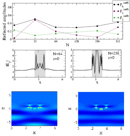
Figure 9: Same as in Fig. 6 but for $\mu=-1.01+i\;10^{-3}$.

5 CONCLUSIONS

We have discussed a number of specific features manifested in numerical simulations of wedges and interfaces of metamaterials, i.e. composite materials with negative dielectric permittivity and negative magnetic permeability. We have demonstrated that a numerical discretization grid in the Yee method may have a dramatic effect on the convergence in numerical modelling of surface waves at interfaces and wedges. In the framework of the continuous-medium approximation, wave scattering on the wedge may result in a resonant excitation of surface waves with infinitely large spatial frequencies, leading to non-convergence of the numerical simulation results that depend strongly on the value of the discretization step. We find that sufficiently high losses may suppress oscillations and allow to obtain converging solutions to the scattering problem, however in the case of smaller losses it may be necessary to take into account the meta-material properties beyond the effective-medium approximation, such as the effect of spatial dispersion.

References

- [1] J. B. Pendry, A. J. Holden, W. J. Stewart, and I. Youngs, “Extremely low frequency plasmons in metallic mesostructures,” Phys. Rev. Lett. 76, 4773–4776 (1996).
- [2] J. B. Pendry, A. J. Holden, D. J. Robbins, and W. J. Stewart, “Magnetism from conductors and enhanced nonlinear phenomena,” IEEE Trans. Microw. Theory Tech. 47, 2075–2084 (1999).
- [3] P. Markos and C. M. Soukoulis, “Numerical studies of left-handed materials and arrays of split ring resonators,” Phys. Rev. E 65, 036622–8 (2002).
- [4] P. Markos and C. M. Soukoulis, “Transmission studies of left-handed materials,” Phys. Rev. B 65, 033401–4 (2002).
- [5] D. R. Smith, W. J. Padilla, D. C. Vier, S. C. Nemat Nasser, and S. Schultz, “Composite medium with simultaneously negative permeability and permittivity,” Phys. Rev. Lett. 84, 4184–4187 (2000).
- [6] M. Bayindir, K. Aydin, E. Ozbay, P. Markos, and C. M. Soukoulis, “Transmission properties of composite metamaterials in free space,” Appl. Phys. Lett. 81, 120–122 (2002).
- [7] C. G. Parazzoli, R. B. Greegor, K. Li, B. E. C. Koltenbah, and M. Tanielian, “Experimental verification and simulation of negative index of refraction using Snell’s law,” Phys. Rev. Lett. 90, 107401–4 (2003).
- [8] V. G. Veselago, “The electrodynamics of substances with simultaneously negative values of and ,” Usp. Fiz. Nauk 92, 517–526 (1967) (in Russian) [English translation: Phys. Usp. 10, 509–514 (1968)].
- [9] J. B. Pendry, “Negative refraction makes a perfect lens,” Phys. Rev. Lett. 85, 3966–3969 (2000).
- [10] N. Fang and X. Zhang, “Imaging properties of a metamaterial superlens,” Appl. Phys. Lett. 82, 161–163 (2003).
- [11] S. A. Cummer, “Simulated causal subwavelength focusing by a negative refractive index slab,” Appl. Phys. Lett. 82, 1503–1505 (2003).
- [12] X. S. Rao and C. K. Ong, “Subwavelength imaging by a left-handed material superlens,” Phys. Rev. E 68, 67601–3 (2003).
- [13] M. W. Feise and Yu. S. Kivshar, “Sub-wavelength imaging with a left-handed material flat lens,” Phys. Lett. A 334, 326–330 (2005).
- [14] N. A. Zharova, I. V. Shadrivov, A. A. Zharov, and Yu. S. Kivshar, “Nonlinear transmission and spatiotemporal solitons in metamaterials with negative refraction,” Optics Express 13, 1291–1298 (2005).
- [15] A. Taflove and S. C. Hagness, Computational Electrodynamics: The Finite-Difference Time-Domain Method, 2nd ed. (Artech House, Norwood, 2000).
- [16] K. S. Yee, “Numerical solution of initial boundary value problems involving Maxwells equations in isotropic media,” IEEE Trans. Antennas Propag. AP14, 302 (1966).
- [17] L. Venema, “Negative refraction: A lens less ordinary,” Nature 420, 119–120 (2002).
- [18] P. Yeh, Optical Waves in Layered Media (John Wiley & Sons, New York, 1988).
- [19] I. V. Shadrivov, A. A. Sukhorukov, and Yu. S. Kivshar, “Guided modes in negative-refractive-index waveguides,” Phys. Rev. E 67, 057602–4 (2003).
- [20] A. D. Boardman, L. Velasco, N. King, and Y. Rapoport, “Ultra-narrow bright spatial solitons interacting with left-handed surfaces,” J. Opt. Soc. Am. B 22, 1443–1452 (2005).
- [21] J. Meixner, “The behavior of electromagnetic fields at edges,” IEEE Trans. Antennas Propag. AP-20, 442–446 (1972).
- [22] G. R. Hadley, “High-accuracy finite-difference equations for dielectric waveguide analysis II: dielectric corners,” J. Lightwave Technol. 20, 1219–1231 (2002).