Maximum-likelihood estimation prevents unphysical Mueller matrices

Abstract

We show that the method of maximum-likelihood estimation, recently introduced in the context of quantum process tomography, can be applied to the determination of Mueller matrices characterizing the polarization properties of classical optical systems. Contrary to linear reconstruction algorithms, the proposed method yields physically acceptable Mueller matrices even in presence of uncontrolled experimental errors. We illustrate the method on the case of an unphysical measured Mueller matrix taken from the literature.

OCIS codes: 000.3860, 260.5430, 290.0290.

In the mathematical description of both polarized light and two-level quantum systems (or qubits, in the language of quantum information), there are many analogies and common tools. For example, the Poincaré sphere BornWolf for classical polarization and the Bloch sphere for two-level quantum systems Feynman are, in fact, the same mathematical object. Although the classical concepts and tools were introduced well before the quantum ones, the latter were developed independently of the former. Thus, many well established results in classical polarization optics have been “rediscovered” in the context of quantum optics and quantum information NielsenBook . Interestingly, the inverse process of borrowing results from quantum to classical optics has started only recently Legre03a ; Brunner03a .

In this Letter we give a contribution to this inverse process by pointing out a connection between quantum process tomography (QPT) Alte03 and classical polarization tomography (CPT). Specifically, we show that the recently introduced maximum-likelihood (ML) method for the estimation of quantum processes Fiura01a ; Sacchi01a ; Kosut04a , can be successfully applied to the determination of classical Mueller matrices. In the conventional approach to CPT, Mueller matrices are estimated from the measurement data by means of linear algorithms LeRoy . However, such reconstructed Mueller matrices often fail to be physically acceptable Anderson94bis . We show that this problem is avoided by using the maximum-likelihood method which allows to include in a natural manner the “physical-acceptability” constraint. Thus, thanks to a “quantum tool”, we solve an important issue that has been long debated in the classical literature Anderson94 ; Gopala98a ; Gopala98b . This is in particular important in view of the present interest in CPT, e.g., for medical and astronomical imaging.

To begin with, we give first a qualitative description of the connection between QPT and CPT. At the heart of this connection lies the well known mathematical equivalence (isomorphism) between the density matrix $\rho$ describing a two-level quantum system and the coherency matrix BornWolf $J$ describing the classical polarization state of a light beam Falkoff51 ; Fano54 :

$$\rho\sim J/\mathrm{Tr}\,J.$$ (1)

$J$ is an Hermitian, positive semidefinite $2\times 2$ matrix, as is $\rho$. A quantum process that transform an input state $\rho^{\mathrm{in}}$ in an output state $\rho^{\mathrm{out}}$ can be described by a linear superoperator $\mathcal{G}:\,\rho^{\mathrm{out}}=\mathcal{G}\rho^{\mathrm{in}}$. Analogously, a classical linear optical process (as, e.g., an elastic scattering process), can be described by a $4\times 4$ matrix $\mathcal{M}$ such that $J^{\mathrm{out}}=\mathcal{M}J^{\mathrm{in}}$ or, in explicit representation,

$$J^{\mathrm{out}}_{ij}=\sum_{k,l}\mathcal{M}_{ij,kl}J^{\mathrm{in}}_{kl},\qquad i,j,k,l\in\{0,1\}.$$ (2)

In the same way as the reconstruction of $\mathcal{G}$ is the goal of QPT, the estimation of the elements $\mathcal{M}_{ij,kl}$ from the measurement data is the goal of CPT. However, in the common practice, instead of the complex matrix elements $\mathcal{M}_{ij,kl}$ one wants to determine the $16$ real elements $M_{\mu\nu},\,(\mu,\nu=0,\ldots,3)$ of the associated Mueller matrix $M$. In the ML approach, the estimated elements of $M$ are found to be the most likely to yield the measured data. In what follows we show how to find them.

In a classical polarization tomography experiment, the measurement data are collected following the scheme shown in Fig. 1.

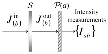
Figure 1: Classical polarization tomography (CPT) scheme.

An input light beam is prepared in a pure polarization state represented by the coherency matrix $J_{(b)}^{\mathrm{in}}$, and sent through the optical system $\mathcal{S}$ where it is transformed in the output beam represented by $J_{(b)}^{\mathrm{out}}=\mathcal{M}J_{(b)}^{\mathrm{in}}$. The estimation strategy is to retrieve information on the system from a series of polarization tests on the output states $J_{(b)}^{\mathrm{out}}$ obtained from distinct input states $J_{(b)}^{\mathrm{in}},\,(b=1,\ldots,B)$. A polarization filter $\mathcal{P}(a)$ that allows the passage of light with specific polarization labelled by the index $a$, $(a=1,\ldots,A)$, provides for the polarization tests. Finally, the intensity $I_{ab}$ of the beam after the filter is recorded. If we prepare $B$ different input states and we perform $A$ polarization tests per each output state, then such a CPT experiment will have $A\times B$ outcomes corresponding to all measured intensities $\{I_{ab}\},\,(a=1,\ldots,A,\,b=1,\ldots,B)$.

However, in a ML approach, which is a probabilistic method, one deals with relative rather than absolute intensities. Therefore, from the data set $\{I_{ab}\}$ we must extract the relative intensities (or measurement frequencies) $f_{ab}=I_{ab}/I_{b}$, where $I_{b}$ is the intensity of the input light beam. Since by definition $0\leq f_{ab}\leq 1$ and $f_{ab}+f_{a^{\prime}b}\leq 1$, where $a,a^{\prime}$ label two mutually orthogonal polarization tests, then $f_{ab}$ provides an experimental estimation of the theoretical probability $p_{ab}$ for obtaining a nonzero output intensity with polarization $a$ when the input beam is prepared in the polarization state $b$. The theoretical probabilities $\{p_{ab}\}$ can be written in terms of the input and output states as MandelBook

$$p_{ab}(\mathcal{M})=\frac{\mathrm{Tr}[\Pi_{(a)}J_{(b)}^{\mathrm{out}}]}{\mathrm{Tr}\,J_{(b)}^{\mathrm{in}}},$$ (3)

where we denoted with $\Pi_{(a)}=\hat{{e}}_{(a)}\otimes\hat{{e}}_{(a)}^{\dagger}$ the $2\times 2$ projection matrix representing the action of the polarization filter $\mathcal{P}(a)$ oriented along the (possibly complex) unit vector $\hat{{e}}_{(a)}$. Since in a CPT experiment the input beam is always prepared in a pure polarization state, it can be represented by a projection matrix $\Pi_{(b)}$ as $J_{(b)}^{\mathrm{in}}=I_{b}\Pi_{(b)}$, where $I_{b}=\mathrm{Tr}\,J_{(b)}^{\mathrm{in}}$ is the intensity of the beam. Then we can rewrite

$$p_{ab}(\mathcal{M})=\mathrm{Tr}[\Pi_{(a)}\mathcal{M}\Pi_{(b)}]\\$$ (4)

where from now on we assume, without loss of generality, $I_{b}=1$. At this point, having measured the frequencies $\{f_{ab}\}$ and having calculated the probabilities $\{p_{ab}\}$, the sought matrix $\mathcal{M}$ can be obtained by maximizing a likelihood function $\mathcal{L}[\mathcal{M}]$ defined as

$$\begin{array}[]{rcl}\mathcal{L}[\mathcal{M}]&=&\displaystyle{\sum_{a,b}f_{ab}\ln[p_{ab}(\mathcal{M})]}\\ &=&\displaystyle{\sum_{a,b}I_{ab}\ln\mathrm{Tr}[\Pi_{(a)}\mathcal{M}\Pi_{(b)}]},\end{array}$$ (5)

where $p_{ab}(\mathcal{M})\geq 0$ for any physically acceptable process.

Equation (5) is the first main result of this paper. It contains both experimental ($I_{ab}$) and theoretical [$p_{ab}(\mathcal{M})$] quantities. Now, we demonstrate that it is possible to impose the condition $p_{ab}(\mathcal{M})\geq 0$ before the maximization operation, in such a way that the estimated Mueller matrix is automatically physically acceptable. After a lengthy but straightforward calculation, it is possible to show that the matrix $\mathcal{M}$ can be written in terms of an Hermitian matrix $H$ as Aiello04d

$$\mathcal{M}=\sum_{\mu,\nu}^{0,3}H_{\mu\nu}\left[\epsilon_{(\mu)}\otimes\epsilon_{(\nu)}\right],$$ (6)

where $\{\epsilon_{(\mu)}\}$ are the elements of the standard basis in $\mathbf{C}^{2\times 2}$. By substituting Eq. (6) into Eq. (3) we obtain

$$p_{ab}(\mathcal{M})=\sum_{\mu,\nu}^{0,3}H_{\mu\nu}\mathrm{Tr}[\Pi_{(a)}\epsilon_{(\mu)}\Pi_{(b)}\epsilon_{(\nu)}^{T}],$$ (7)

where the superscript $T$ indicates the transposed matrix. The probabilities $p_{ab}(\mathcal{M})$ as written in Eq. (7) can still be negative, because only $H$ matrices associated with physically acceptable Mueller matrices can guarantee the condition $p_{ab}\geq 0$. However, we know from the Mueller matrix theory that the $H$ matrix associated with a physically acceptable Mueller matrix must be positive semidefinite Anderson94 . It is well known that any positive semidefinite matrix can be written in terms of its Cholesky decomposition as

$$H=2\frac{CC^{\dagger}}{\mathrm{Tr}(CC^{\dagger})},$$ (8)

where $C$ is a lower triangular matrix

$$C=\begin{pmatrix}h_{1}&0&0&0\\ h_{5}+\mathrm{i}h_{6}&h_{2}&0&0\\ h_{11}+\mathrm{i}h_{12}&h_{7}+\mathrm{i}h_{8}&h_{3}&0\\ h_{15}+\mathrm{i}h_{16}&h_{13}+\mathrm{i}h_{14}&h_{9}+\mathrm{i}h_{10}&h_{4}\end{pmatrix},$$ (9)

composed by $16$ real parameters $h_{k},\,(k=1,\ldots,16)$, and we fixed the normalization of $H$ by setting $M_{00}=1$. Then, after substituting Eq. (8) into Eq. (7), the maximum of $\mathcal{L}$ can be found by using a standard maximization algorithm RecipeFor . The search for the maximum is performed in the real $16$-dimensional space of parameters $\{h_{k}\}$. Once the optimal set of values $\{h_{1}^{\mathrm{opt}},\ldots,h_{16}^{\mathrm{opt}}\}$ that maximize $\mathcal{L}$ has been found, this can be used in Eq. (8) to obtain the corresponding $H^{\mathrm{opt}}$. Finally, the elements of the sought physically acceptable Mueller matrix can be computed as

$$M_{\mu\nu}=\mathrm{Tr}\left\{H^{\mathrm{opt}}[\sigma_{(\mu)}\otimes\sigma_{(\nu)}^{*}]\right\},$$ (10)

where $\{\sigma_{(\mu)}\}$ are the normalized Pauli matrices Aiello04d . This is our second main result. A Mueller matrix $M$ determined in this way represents the answer to the question: “which physically acceptable Mueller matrix is most likely to yield the measured data? ”

The rest of the paper is devoted to the illustration of the theory outlined above, by applying it to a realistic case. We have chosen from the current literature Howell the following Mueller matrix which was already shown Anderson94 to be physically unacceptable:

$$M^{\prime}=\begin{pmatrix}{0.7599}&{0.0295}&{0.1185}&-\text{0.0623}\\ {0.0384}&{0.5394}&{0.0282}&-\text{0.1714}\\ {0.124}&-\text{0.012}&{0.6608}&{0.2168}\\ -\text{0.0573}&-\text{0.1811}&-\text{0.1863}&{0.4687}\end{pmatrix}.$$ (11)

From $M^{\prime}$ we calculated the (normalized) associated Hermitian matrix $H^{\prime}$ which is not positive semidefinite since it has one negative eigenvalue:

$$\mathrm{diag}\,H^{\prime}=\{1.6671,\,0.2950,\,0.2330,\,-0.1951\}.$$ (12)

By using Eq. (7), we generated a set of $36$ “fake-measured” data $f_{ab}^{\prime}$ as

$$f_{ab}^{\prime}=\sum_{\mu,\nu}^{0,3}H_{\mu\nu}^{\prime}\mathrm{Tr}[\Pi_{(a)}\epsilon_{(\mu)}\Pi_{(b)}\epsilon_{(\nu)}^{T}],$$ (13)

where we selected both the input beam (represented by $\Pi_{(b)}$) and the polarization filter (represented by $\Pi_{(a)}$) from the set of $6$ pure polarization states labelled as horizontal (H) and vertical (V), oblique at $45^{\circ}$ and oblique at $135^{\circ}$, right (RHC) and left (LHC). The so obtained $36$ numbers represent our “experimental” data set. Obviously, from these numbers one could generate back $M^{\prime}$ with the conventional linear algorithm. It may worth to note that the three pairs of polarization states we have chosen, are the ones usually employed in CPT BornWolf , and correspond to three mutually unbiased basis PeresBook often utilized in QPT. We used the MATHEMATICA 5.1 function FindMaximum to maximize $\mathcal{L}$. Tho run this function it is necessary to furnish a set of initial values for the parameters $\{h_{1},\ldots,h_{16}\}$ to be estimated. We found convenient to proceed in the following way: we made first a polar decomposition of $H^{\prime}$ to obtain the positive semidefinite matrix $H^{\prime\prime}=2\sqrt{H^{\prime}{H^{\prime}}^{\dagger}}/\mathrm{Tr}\sqrt{H^{\prime}{H^{\prime}}^{\dagger}}$, then we obtain the initial values from the Cholesky decomposition of $H^{\prime\prime}$. Finally, after maximization, we obtained the maximum-likelihood estimation of $M^{\mathrm{ML}}$ as

$$M^{\mathrm{ML}}=\begin{pmatrix}\text{0.7599}&\text{0.0257}&\text{0.1206}&-\text{0.0576}\\ \text{0.0372}&\text{0.5285}&\text{0.0001}&-\text{0.0496}\\ \text{0.1208}&-\text{0.0001}&\text{0.6184}&\text{0.1920}\\ -\text{0.0554}&-\text{0.0572}&-\text{0.1794}&\text{0.4822}\end{pmatrix}.$$ (14)

As expected, this matrix is indeed a physically acceptable Mueller matrix, as the eigenvalues of its associated $H^{\mathrm{ML}}$ matrix are all non-negative:

$$\mathrm{diag}\,H^{\mathrm{ML}}=\{1.6344,\,0.2341,\,0.1315,\,0\}.$$ (15)

A visual inspection show that $M$ and $M^{\mathrm{ML}}$ differs only by a little amount. This was expected since we choose an initial Mueller matrix $M^{\prime}$ that is not very unphysical (only one negative eigenvalue ). A quantitative estimation of the difference between $M^{\prime}$ and $M^{\mathrm{ML}}$ can be given by calculating their relative Frobenius distance LeRoy

$$\frac{||M-M^{\mathrm{ML}}||}{||M+M^{\mathrm{ML}}||}=0.072,$$ (16)

which indicates that the average relative difference between corresponding matrix elements of $M$ and $M^{\mathrm{ML}}$ is about $7\%$. This confirms the quality of our approach even with sparse data set (only 36 values).

In conclusion, we have shown that it is possible to apply the maximum-likelihood method, initially developed for quantum process tomography, to the classical problem of Mueller matrix reconstruction. Moreover, we have shown that this method has the benefit to produce always physically acceptable Mueller matrices as the most likely matrices which yield the measured data.

We acknowledge support from the EU under the IST-ATESIT contract. This project is also supported by FOM.

References

- (1) M. Born and E. Wolf. Principles of Optics, 7th expanded edition, (Cambridge University Press, 1999).
- (2) R. P. Feynamn, F. L. Vernon Jr., and R. W. Hellwarth, J. Appl. Phys. 28, 49 (1957).
- (3) M. A. Nielsen and I. L. Chuang, Quantum Computation and Quantum Information, reprinted first edition, (Cambridge University Press, Cambridge, UK, 2002).
- (4) M. Legré, M. Wegmüller, and N. Gisin, Phys. Rev. Lett. 91, 167902 (2003).
- (5) N. Brunner, A. Acín, D. Collins, N. Gisin, and V. Scarani, Phys. Rev. Lett. 91, 180402 (2003).
- (6) J. B. Altepeter et al., Phys. Rev. Lett. 90, 193601 (2003).
- (7) J. Fiurášek and Z. Hradil, Phys. Rev. A 63, 020101(R) (2001).
- (8) M. F. Sacchi, Phys. Rev. A 63, 054104 (2001).
- (9) R. L. Kosut, I. Walmsley, and H. Rabitz, arXiv, quant-ph/0411093.
- (10) F. Le Roy-Brehonnet and B. Le Jeune, Prog. Quant. Electr. 21, 109 (1997).
- (11) In the current literature there is some confusion in the use of terms such as “nominal” Mueller matrix, “physical” Mueller matrix, etc.. Here we adopt the terminology of Ref. Anderson94 .
- (12) D. G. M. Anderson and R. Barakat, J. Opt. Soc. Am. A 11, 2305 (1994).
- (13) A. V. Gopala Rao, K. S. Mallesh, and Sudha, J. Mod. Opt. 45, 955 (1998).
- (14) A. V. Gopala Rao, K. S. Mallesh, and Sudha, J. Mod. Opt. 45, 989 (1998).
- (15) D. L. Falkoff and J. E. McDonald, J. Opt. Soc. Am. 41, 862 (1951).
- (16) U. Fano, Phys. Rev. 93, 121 (1954).
- (17) L. Mandel and E. Wolf, Optical Coherence and Quantum Optics, first edition, (Cambridge University Press, 1995).
- (18) A. Aiello, and J. P. Woerdman, math-ph/0412061 (2004).
- (19) W. H. Press, S. A. Teukolsky, W. T. Vetterling, and B. P. Flannery, Numerical Recipes in FORTRAN, second edition, (Cambridge University Press, 1994).
- (20) B. J. Howell, Appl. Opt. 18, 1809 (1979).
- (21) A. Peres, Quantum Theory, Concepts and Methods. (Kluwer Academic Publisher, 1998).