Rutherford scattering with radiation damping

Abstract

We study the effect of radiation damping on the classical scattering of charged particles. Using a perturbation method based on the Runge-Lenz vector, we calculate radiative corrections to the Rutherford cross section, and the corresponding energy and angular momentum losses.

1 Introduction

The reaction of a classical point charge to its own radiation was first discussed by Lorentz and Abraham more than one hundred years ago, and never stopped being a source of controversy and fascination [1, 2, 3, 4]. Nowadays, it is probably fair to say that the most disputable aspects of the Lorentz-Abraham-Dirac theory, like runaway solutions and preacceleration, have been adequately understood and treated in terms of finite-size effects (for a review see Ref. [4]). In any case, radiation damping considerably complicates the equations of motion of charged particles, and for many basic problems, like Rutherford scattering, only numerical calculations of the trajectories are available [5, 6]. In this paper we study the effect of radiation reaction on the classical two-body scattering of charged particles. Following Landau and Lifshitz [2], we expand the electromagnetic force in powers of $c^{-1}$ ($c$ is the speed of light), up to the order $c^{-3}$ where radiation damping appears. Then, using a perturbation technique based on the Runge-Lenz vector [7], we calculate the radiation damping corrections to the Rutherford deflection function and scattering cross section, and the corresponding expressions for the angular momentum and energy losses.

This paper is organized as follows. In Sec. 2 we obtain the radiation damping force on a system of charged particles, from the expansion of the electromagnetic field in powers of $1/c$. The equations of motion for a two-body system with radiation reaction are discussed in Sec. 3, and in Sec. 4 we use the Runge-Lenz vector to calculate the radiation effect on classical Rutherford scattering. Some final remarks are made in Sec. 5.

2 The radiation damping force

In this section we reproduce, for completeness, the derivation of the radiation damping force given by Landau and Lifshitz [2]. We start from the electromagnetic potentials $\phi({\bf r},t)$ and ${\bf\cal A}({\bf r},t)$, created by the charge and current densities $\rho({\bf r},t)$ and ${\bf J}({\bf r},t)$,

$$\phi({\bf r},t)=\int{\rho({\bf r}^{\prime},t_{R})\over R}d^{3}{\bf r}^{\prime}\,,$$ (1)

$${\bf\cal A}({\bf r},t)=\frac{1}{c}\int{{\bf J}({\bf r}^{\prime},t_{R})\over R}d^{3}{\bf r}^{\prime}\,.$$ (2)

Here, $R=|{\bf r}-{\bf r}^{\prime}|$ and $t_{R}=t-R/c$ is the retarded time. The electric and magnetic fields, ${\bf E}$ and ${\bf B}$, are obtained from the potentials as

$${\bf E}=-\nabla\phi({\bf r},t)-\frac{1}{c}{\partial{\bf\cal A}({\bf r},t)\over\partial t}\ \ \ ,\ \ \ {\bf B}=\nabla\times{\bf\cal A}({\bf r},t)\ .$$ (3)

We want to calculate the electromagnetic force on a charge $q$,

$${\bf F}=q{\bf E}+{q\over c}{\bf v}\times{\bf B},$$ (4)

as a series in powers of $1/c$. In order to do this, we expand $\rho({\bf r}^{\prime},t_{R})$ and ${\bf J}({\bf r}^{\prime},t_{R})$ in Taylor series around $t_{R}=t$,

$$\rho({\bf r}^{\prime},t_{R}) = \rho({\bf r}^{\prime},t)+\frac{\partial\rho({\bf r}^{\prime},t)}{\partial t}\left(-\frac{R}{c}\right)+\frac{1}{2}\frac{\partial^{2}\rho({\bf r}^{\prime},t)}{\partial t^{2}}\left(-\frac{R}{c}\right)^{2}$$ (6)

$$+\frac{1}{6}\frac{\partial^{3}\rho({\bf r}^{\prime},t)}{\partial t^{3}}\left(-\frac{R}{c}\right)^{3}+{\cal O}(c^{-4})\,,$$

$${\bf J}({\bf r}^{\prime},t_{R}) = {\bf J}({\bf r}^{\prime},t)+\frac{\partial{\bf J}({\bf r}^{\prime},t)}{\partial t}\left(-\frac{R}{c}\right)+{\cal O}(c^{-2})\,.$$ (7)

Substituting these expansions in Eqs.(1) and (2), and noting the charge conservation relation,

$$\frac{\partial}{\partial t}\int\rho({\bf r}^{\prime},t)d^{3}{\bf r}^{\prime}=0\,,$$ (8)

we obtain

$$\phi({\bf r},t) = \int\frac{\rho({\bf r}^{\prime},t)}{R}d^{3}{\bf r}^{\prime}+\frac{1}{2c^{2}}\frac{\partial^{2}}{\partial t^{2}}\int R\rho({\bf r}^{\prime},t)d^{3}{\bf r}^{\prime}$$ (10)

$$-\frac{1}{6c^{3}}\frac{\partial^{3}}{\partial t^{3}}\int R^{2}\rho({\bf r}^{\prime},t)d^{3}{\bf r}^{\prime}+{\cal O}(c^{-4})$$

$$\frac{1}{c}{\bf\cal A}({\bf r},t) = \frac{1}{c^{2}}\int{{\bf J}({\bf r}^{\prime},t)\over R}d^{3}{\bf r}^{\prime}-\frac{1}{c^{3}}{\partial\over\partial t}\int{\bf J}({\bf r}^{\prime},t)d^{3}{\bf r}^{\prime}+{\cal O}(c^{-4})\,.$$ (11)

With the gauge transformation

$$\phi({\bf r},t) \rightarrow \phi({\bf r},t)-\frac{1}{c}{\partial\chi({\bf r},t)\over\partial t}$$ (12)

$${\bf\cal A}({\bf r},t) \rightarrow {\bf\cal A}({\bf r},t)+{\bf\nabla}\chi({\bf r},t)\ ,$$ (14)

where

$$\chi({\bf r},t)={1\over 2c}{\partial\over\partial t}\int R\rho({\bf r},t)\ d^{3}{\bf r}^{\prime}-{1\over 6c^{2}}{\partial^{2}\over\partial t^{2}}\int R^{2}\rho({\bf r},t)\ d^{3}{\bf r}^{\prime}\ ,$$ (15)

we can rewrite Eqs. (10) and (11) as

$$\phi({\bf r},t) = \int{\rho({\bf r}^{\prime},t)\over R}d^{3}{\bf r}^{\prime}+{\cal O}(c^{-4})$$ (16)

$$\frac{1}{c}{\bf\cal A}({\bf r},t) = \frac{1}{c^{2}}\int{{\bf J}({\bf r}^{\prime},t)\over R}d^{3}{\bf r}^{\prime}+\frac{1}{2c^{2}}{\partial\over\partial t}\int\frac{\bf R}{R}\rho({\bf r}^{\prime},t)d^{3}{\bf r}^{\prime}$$ (18)

$$-\frac{1}{c^{3}}{\partial\over\partial t}\int{\bf J}({\bf r}^{\prime},t)d^{3}{\bf r}^{\prime}-\frac{1}{3c^{3}}{\partial^{2}\over\partial t^{2}}\int{\bf R}\rho({\bf r}^{\prime},t)d^{3}{\bf r}^{\prime}+{\cal O}(c^{-4})\,.$$

For a set of point charges $q_{k}$, with positions ${\bf r}_{k}(t)$ and velocities ${\bf v}_{k}(t)$, we have

$$\rho({\bf r},t) = \sum_{k}q_{k}\delta\Bigl{(}{\bf r}-{\bf r}_{k}(t)\Bigr{)}\,,$$ (19)

$${\bf J}({\bf r},t) = \sum_{k}q_{k}{\bf v}_{k}(t)\delta\Bigl{(}{\bf r}-{\bf r}_{k}(t)\Bigr{)}\,,$$ (20)

and the potentials become

$$\phi({\bf r},t) = \sum_{k}{q_{k}\over R_{k}(t)}+{\cal O}(c^{-4})$$ (21)

$$\frac{1}{c}{\bf\cal A}({\bf r},t) = \frac{1}{c^{2}}\sum_{k}{q_{k}{\bf v}_{k}(t)\over R_{k}(t)}+{1\over 2c^{2}}{d\over dt}\sum_{k}{{\bf R}_{k}(t)\over R_{k}(t)}q_{k}$$ (23)

$$-{1\over c^{3}}{d\over dt}\sum_{k}{q_{k}{\bf v}_{k}(t)}-{1\over 3c^{3}}{d^{2}\over dt^{2}}\sum_{k}{\bf R}_{k}(t)q_{k}+{\cal O}(c^{-4})\,,$$

with ${\bf R}_{k}(t)={\bf r}-{\bf r}_{k}(t)$. Carrying out the time derivatives in Eq. (23) we obtain

$$\frac{1}{c}{\bf\cal A}({\bf r},t) = {1\over 2c^{2}}\sum_{k}\left[{q_{k}{\bf v}_{k}(t)\over R_{k}(t)}+{q_{k}{\bf R}_{k}(t).{\bf v}_{k}(t)\over R_{k}^{3}(t)}{\bf R}_{k}(t)\right]$$ (25)

$$-{2\over 3c^{3}}\sum_{k}q_{k}{\bf a}_{k}(t)+{\cal O}(c^{-4})\,,$$

where ${\bf a}_{k}(t)$ is the acceleration of particle $k$.

The $\phi$ potential given in Eq. (21) accounts for the Coulomb interaction. The first term in Eq. (25), of order $1/c^{2}$, introduces magnetic and retardation effects, and can be used to set up the Darwin lagrangian [2]. The last term in Eq. (25), of order $1/c^{3}$, gives the radiation damping electric field

$${\bf E}_{rd}={2\over 3c^{3}}\sum_{k}q_{k}\frac{d{\bf a}_{k}}{dt}\,,$$ (26)

and a null magnetic field ($\bf\cal A$ is independent of $\bf r$ in this order). Introducing the electric dipole of the system, ${\bf D}=\sum_{k}q_{k}{\bf r}_{k}$, the radiation damping field of Eq. (26) can be written as

$${\bf E}_{rd}=\frac{2}{3c^{3}}\frac{d^{3}{\bf D}}{dt^{3}}\,,$$ (27)

showing that it represents the reaction to the electric dipole radiation emitted by the whole system.

The radiation damping force on charge $q_{i}$ is then

$${\bf F}^{(i)}_{rd}={q_{i}\bf E}_{rd}={2\over 3c^{3}}\sum_{k}q_{i}q_{k}\frac{d{\bf a}_{k}}{dt}\,.$$ (28)

It should be stressed that radiation reaction is not just a self-force — it gets contributions from every particle in the system. Only for a single accelerating charge $q$ the radiation damping force reduces to the Abraham-Lorentz self-interaction

$${\bf F}_{rd}={2\over 3}{q^{2}\over c^{3}}\frac{d{\bf a}}{dt}\ .$$ (29)

3 Two-body motion with radiation damping

Let us consider a system of two charged particles. Taking radiation damping into account, their equations of motion read

$${d^{2}{\bf r}_{1}\over dt^{2}} = \frac{q_{1}q_{2}}{m_{1}}\frac{\bf r}{r^{3}}+{2\over 3c^{3}}{q_{1}\over m_{1}}\frac{d}{dt}(q_{1}{\bf{a}}_{1}+q_{2}{\bf{a}}_{2})\,,$$ (30)

$${d^{2}{\bf r}_{2}\over dt^{2}} = -\frac{q_{1}q_{2}}{m_{2}}\frac{\bf r}{r^{3}}+{2\over 3c^{3}}{q_{2}\over m_{2}}\frac{d}{dt}(q_{1}{\bf{a}}_{1}+q_{2}{\bf{a}}_{2})\,.$$ (31)

where ${\bf r}={\bf r}_{1}-{\bf r}_{2}$ and $m_{i}$ is the mass of particle $i$. In these equations we have discarded the $c^{-2}$ terms that account for the variation of mass with velocity and the Darwin magnetic and retardation effects. These terms do not interfere with our treatment of radiation damping, and their effect on Rutherford scattering is discussed in Refs. [7, 8].

Subtracting Eq. (31) from (30) we find

$${d^{2}{\bf r}\over dt^{2}}={q_{1}q_{2}\over\mu}{{\bf r}\over r^{3}}+{2\over 3c^{3}}\biggl{(}{q_{1}\over m_{1}}-{q_{2}\over m_{2}}\biggr{)}\frac{d}{dt}(q_{1}{\bf{a}}_{1}+q_{2}{\bf{a}}_{2})\,,$$ (32)

where $\mu=m_{1}m_{2}/(m_{1}+m_{2})$ is the reduced mass. From equations (30), (31) and (32), it is easily shown that, keeping only the lowest order ($c^{0}$) terms,

$$q_{1}{\bf{a}}_{1}+q_{2}{\bf{a}}_{2}=\mu\left({q_{1}\over m_{1}}-{q_{2}\over m_{2}}\right){d^{2}{\bf r}\over dt^{2}}\,.$$ (33)

Substituting this result in Eq. (32) we obtain

$${d^{2}{\bf r}\over dt^{2}}={q_{1}q_{2}\over\mu}{{\bf r}\over r^{3}}+\frac{2\tilde{q}^{2}}{3\mu c^{3}}\frac{d^{3}{\bf r}}{dt^{3}}\,,$$ (34)

where

$$\tilde{q}=\mu\biggl{(}{q_{1}\over m_{1}}-{q_{2}\over m_{2}}\biggr{)}\ .$$ (35)

In the fixed target limit, $m_{2}\to\infty$, Eq. (34) becomes the nonrelativistic Lorentz-Abraham equation of motion. It is interesting to see that two-body recoil effects appear in Eq. (34) not only through the reduced mass $\mu$, but also via the effective charge $\tilde{q}$. In particular, if $q_{1}/m_{1}=q_{2}/m_{2}$ we have $\tilde{q}=0$, and there is no radiation reaction even though both particles are accelerating. This is related to the fact that, in this case, there is no electric dipole radiation from the system.

4 Radiative correction to Rutherford scattering

In the absence of perturbations, Rutherford scattering conserves the total energy $E=\frac{1}{2}\mu v^{2}+q_{1}q_{2}/r$, the angular momentum ${\bf L}=\mu{\bf r}\times{\bf v}$, and the Runge-Lenz vector [9]

$${\bf A}={\bf v}\times{\bf L}+q_{1}q_{2}\,{\bf\hat{r}}\,.$$ (36)

Here, ${\bf v}=d{\bf r}/dt$ is the relative velocity and ${\bf\hat{r}}={\bf r}/r$ is the radial unit vector. These conserved quantities are not independent: it is easily seen that ${\bf A}\cdot{\bf L}=0$ and

$$A^{2}=2EL^{2}/\mu+(q_{1}q_{2})^{2}=(v_{0}L)^{2}+(q_{1}q_{2})^{2}\,,$$ (37)

where $v_{0}$ is the initial (asymptotic) velocity. Taking the scalar product ${\bf r}\cdot{\bf A}$, one finds the Rutherford scattering orbit

$$r(\varphi)=\frac{L^{2}/\mu}{A\cos\varphi-q_{1}q_{2}}\,,$$ (38)

where $\varphi$ is the angle between ${\bf r}$ and ${\bf A}$. During the collision, $\varphi$ changes from $-\varphi_{0}$ to $\varphi_{0}$, where

$$\varphi_{0}=\cos^{-1}(q_{1}q_{2}/A)=\tan^{-1}(v_{0}L/q_{1}q_{2})\,.$$ (39)

The scattering angle is $\theta=\pi-2\varphi_{0}$, and from Eq. (39) we obtain the Rutherford deflection function

$$\theta(L)=2\tan^{-1}(q_{1}q_{2}/v_{0}L)\,.$$ (40)

Note that for charges of the same sign the scattering angle is positive, and for opposite charges $\theta$ is negative (we take $L$ and $v_{0}$ as always positive).

When radiation damping is considered, $E$, ${\bf L}$ and ${\bf A}$ are no longer conserved. In particular, from Eq. (34) we can show that the Runge-Lenz vector changes at the rate

$$\frac{d{\bf A}}{dt}=\frac{2\tilde{q}^{2}}{3c^{3}}\left[\frac{1}{\mu}\frac{d^{3}{\bf r}}{dt^{3}}\times{\bf L}+{\bf v}\times\left({\bf r}\times\frac{d^{3}{\bf r}}{dt^{3}}\right)\right]\,.$$ (41)

The total change of ${\bf A}$ during the collision is then

$$\delta{\bf A}=\frac{2\tilde{q}^{2}}{3c^{3}}\int_{-\infty}^{\infty}dt\left[\frac{1}{\mu}\frac{d^{3}{\bf r}}{dt^{3}}\times{\bf L}+{\bf v}\times\left({\bf r}\times\frac{d^{3}{\bf r}}{dt^{3}}\right)\right]\,.$$ (42)

The change of the Runge-Lenz vector is of order $c^{-3}$. Keeping the same order of approximation, we can substitute in the integrand of Eq. (42) the results of unperturbed Rutherford scattering. We obtain

$$\delta{\bf A}=\frac{2\tilde{q}^{2}}{3c^{3}}\frac{q_{1}q_{2}}{\mu^{2}}\int_{-\infty}^{\infty}dt\frac{{\bf A}-q_{1}q_{2}\,{\bf\hat{r}}}{r^{3}}\,,$$ (43)

which is further simplified by a change of variable from time $t$ to angle $\varphi$. Still working to order $c^{-3}$, we have

$$dt=\frac{\mu r^{2}}{L}d\varphi\,,$$ (44)

and

$$\delta{\bf A}=\frac{2\tilde{q}^{2}}{3c^{3}}\frac{q_{1}q_{2}}{\mu L}\int_{-\varphi_{0}}^{\varphi_{0}}d\varphi\frac{{\bf A}-q_{1}q_{2}\,{\bf\hat{r}}}{r}\,.$$ (45)

Substituting $r(\varphi)$ from Eq. (38), the above integral reduces to

$$\delta{\bf A}=\frac{2\tilde{q}^{2}}{3c^{3}}\frac{q_{1}q_{2}}{{L}^{3}A}{\bf A}\int_{-\varphi_{0}}^{\varphi_{0}}d\varphi\left(A\cos\varphi-q_{1}q_{2}\right)\left(A-q_{1}q_{2}\cos\varphi\right)\,,$$ (46)

which is easily calculated. Using Eq. (39), the result is written as

$$\delta{\bf A}=\frac{2\tilde{q}^{2}}{3c^{3}}\frac{q_{1}q_{2}v_{0}}{L^{2}}\left[2+\frac{1}{1+(v_{0}L/q_{1}q_{2})^{2}}-3\frac{q_{1}q_{2}}{v_{0}L}\tan^{-1}(v_{0}L/q_{1}q_{2})\right]{\bf A}\,.$$ (47)

According to Eq. (39), the change in the Runge-Lenz vector modifies the asymptotic angle $\varphi_{0}$ by

$$\delta\varphi_{0}=\frac{q_{1}q_{2}}{v_{0}L}\,\frac{\delta A}{A}\,,$$ (48)

and the scattering angle $\theta$ by (see Ref. [7])

$$\delta\theta=-\delta\varphi_{0}\,.$$ (49)

The deflection function is then given as

$$\theta(L)=2\tan^{-1}(q_{1}q_{2}/v_{0}L)+\delta\theta(L)$$ (50)

where the first term is the Rutherford relation, and the radiation damping correction is

$$\delta\theta(L)=-\frac{2\tilde{q}^{2}}{3c^{3}}\frac{(q_{1}q_{2})^{2}}{L^{3}}\left[2+\frac{1}{1+(v_{0}L/q_{1}q_{2})^{2}}-3\frac{q_{1}q_{2}}{v_{0}L}\tan^{-1}(v_{0}L/q_{1}q_{2})\right]\,.$$ (51)

From these equations we can also obtain $L(\theta)$. To order $c^{-3}$, the result is

$$L(\theta)=\frac{q_{1}q_{2}}{v_{0}}\cot(\theta/2)\left[1+\frac{\tilde{q}^{2}}{q_{1}q_{2}}\left(\frac{v_{0}}{c}\right)^{3}\lambda(\theta)\right]\,,$$ (52)

where

$$\lambda(\theta)=\frac{1}{6}\frac{\sin^{3}(\theta/2)}{\cos^{5}(\theta/2)}\left[(5-\cos\theta)\cot(\theta/2)-3(\pi-\theta)\right]\,.$$ (53)

A plot of $\lambda(\theta)$ is shown in Fig. 1. As already mentioned, positive angles are reached by like-sign charges, and negative angles by oppositely charged particles. We see that the radiative correction is limited if the Coulomb force is repulsive, and is strongly divergent for backscattering ($\theta\rightarrow-\pi$) in an attractive Coulomb field.

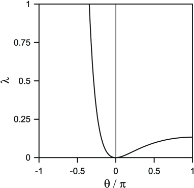
Figure 1: Angular dependence of the radiative correction to Rutherford’s deflection function. Positive (negative) angles correspond to the scattering of like (unlike) charges.

The scattering cross section can be calculated from the deflection as

$$\frac{d\sigma}{d\Omega}=\frac{1}{p^{2}}\left|\frac{L}{\sin\theta}\frac{dL}{d\theta}\right|\,,$$ (54)

where $p=\mu v_{0}$ is the initial momentum. With Eqs. (52) and (53) we get

$$\frac{d\sigma}{d\Omega}=\frac{d\sigma_{R}}{d\Omega}\left[1+\frac{\tilde{q}^{2}}{q_{1}q_{2}}\left(\frac{v_{0}}{c}\right)^{3}\xi(\theta)\right]\,,$$ (55)

where

$$\frac{d\sigma_{R}}{d\Omega}=\left(\frac{q_{1}q_{2}}{2\mu{v_{0}}^{2}}\right)^{2}\frac{1}{\sin^{4}(\theta/2)}$$ (56)

is the nonrelativistic Rutherford cross section, and

$$\xi(\theta)=\frac{1}{2}\frac{\sin^{3}(\theta/2)}{\cos^{5}(\theta/2)}\left[(\pi-\theta)(2-\cos\theta)-3\sin\theta\right]\,.$$ (57)

The function $\xi(\theta)$ is shown in Fig. 2. At large angles, close to backscattering, $\xi(\theta)$ has the limits

$$\xi(\theta) \sim \frac{4}{15}-\frac{2}{35}(\theta-\pi)^{2}+\dots\qquad(\theta\rightarrow\pi)$$ (58)

$$\xi(\theta) \sim -96\pi(\theta+\pi)^{-5}+\dots\qquad(\theta\rightarrow-\pi)$$ (59)

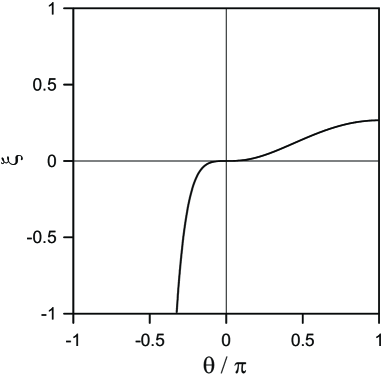
Figure 2: Angular dependence of the radiative correction to the Rutherford cross section. Positive/negative angles are the same as in Fig. 1.

The angular momentum loss (or gain) can be calculated with similar methods. With radiation damping, the time derivative of ${\bf L}$ is given by

$$\frac{d{\bf L}}{dt}=\frac{2\tilde{q}^{2}}{3c^{3}}\,{\bf r}\times\frac{d^{3}{\bf r}}{dt^{3}}\,,$$ (60)

which, integrated on the unperturbed Rutherford trajectory, gives the total change of angular momentum in the scattering process,

$$\delta{\bf L}=\frac{4{\tilde{q}}^{2}}{3c^{3}}\frac{q_{1}q_{2}v_{0}}{L^{2}}\left[1-\frac{q_{1}q_{2}}{v_{0}L}\arctan\left(\frac{v_{0}L}{q_{1}q_{2}}\right)\right]{\bf L}\,.$$ (61)

At a given scattering angle, the angular momentum change is

$$\delta{\bf L}=\frac{4}{3}\frac{{\tilde{q}}^{2}}{q_{1}q_{2}}\left(\frac{v_{0}}{c}\right)^{3}\chi(\theta)\,{\bf L}$$ (62)

where

$$\chi(\theta)=\tan^{2}(\theta/2)\left[1-\frac{\pi-\theta}{2}\tan(\theta/2)\right]\,.$$ (63)

This function is shown in Fig. 3

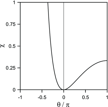
Figure 3: Angular dependence of the change in angular momentum. Positive/negative angles are the same as in Fig. 1.

The energy loss is readily calculated by differentiating Eq. (37),

$$\frac{\delta E}{E}=\frac{2}{(v_{0}L)^{2}}{\bf A}\cdot{\delta{\bf A}}-\frac{2}{L^{2}}{\bf L}\cdot{\delta{\bf L}}\,.$$ (64)

Inserting the expressions for $\delta{\bf A}$ and $\delta{\bf L}$ we obtain

$$\frac{\delta E}{E}=\frac{4{\tilde{q}}^{2}}{3c^{3}}\frac{(q_{1}q_{2})^{2}}{L^{3}}\left\{3\frac{q_{1}q_{2}}{v_{0}L}-\left[1+3\left(\frac{q_{1}q_{2}}{v_{0}L}\right)^{2}\right]\arctan\left(\frac{v_{0}L}{q_{1}q_{2}}\right)\right\}\,,$$ (65)

or, in terms of the scattering angle,

$$\frac{\delta E}{E}=-\frac{4}{3}\frac{{\tilde{q}}^{2}}{q_{1}q_{2}}\left(\frac{v_{0}}{c}\right)^{3}\xi(\theta)\,$$ (66)

where $\xi(\theta)$ is the same function given in Eq. (57) and shown in Fig. 2.

5 Final comments

Our discussion of radiation damping corrections to Rutherford scattering ignored relativistic effects like retardation, magnetic forces, and the mass-velocity dependence. These effects give contributions of order $c^{-2}$ to the deflection function and cross section (see Ref. [7]), and are generally more important than the $c^{-3}$ radiative corrections we have obtained. They were not considered here because, as already mentioned, this would not change our results: a $c^{-2}$ correction to the nonrelativistic Rutherford trajectory only adds $c^{-5}$ terms to our perturbative calculation of radiation damping. We can easily write the complete (up to $c^{-3}$) expansion of the deflection function and scattering cross section by putting together the results of Ref. [7] and the present paper. For example, the differential cross section to order $c^{-3}$ reads

$$\frac{d\sigma}{d\Omega}=\frac{d\sigma_{R}}{d\Omega}\left[1-\left(\frac{v_{0}}{c}\right)^{2}h(\theta)\right]\left[1+5\frac{\mu}{M}\left(\frac{v_{0}}{c}\right)^{2}\right]\left[1+\frac{\tilde{q}^{2}}{q_{1}q_{2}}\left(\frac{v_{0}}{c}\right)^{3}\xi(\theta)\right]\,,$$ (67)

where

$$h(\theta)=\frac{1}{2}\tan^{2}(\theta/2)\left[1+(\pi-\theta)\cot\theta\right]+1$$ (68)

and $M=m_{1}+m_{2}$. As discussed in [7], the first corrective term accounts for the variation of mass with velocity, and the second includes magnetic and retardation effects. The last one is the radiative correction calculated in the previous section. It is interesting to note that magnetic and retardation effects simply renormalize the cross section by an angle independent factor.

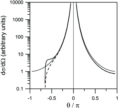
Figure 4: Rutherford scattering to order $c^{-3}$. The projectile velocity is $0.4\,c$, and the target has infinite mass. The two electric charges are of the same magnitude, like (unlike) signs corresponding to positive (negative) scattering angles. The nonrelativistic Rutherford cross section is given by the dotted lines. The dashed lines incorporate $c^{-2}$ corrections, and the solid lines include the $c^{-3}$ radiation damping effects.

In Fig. 4 we show the differential cross section for the scattering of a charged particle with $v_{0}=0.4\,c$ on a fixed target, of equal ($\theta>0$) or opposite ($\theta<0$) charge. The dotted lines give the nonrelativistic cross section, and the dashed ones show the effect of the $c^{-2}$ relativistic mass correction (retardation and magnetic forces do not show up on a fixed target). The solid lines bring in the radiation damping effect, as given in Eq. (67). We see in Fig. 4 that radiation damping has a very small effect when the charges repel each other. But for an attractive Coulomb force the radiative correction is quite important (as also seen in Fig. 2), creating a plateau-like structure in the angular distribution. Even though our perturbative results are not reliable for large corrections, such structure is very similar to what is found in “exact” numerical calculations [6].

A final point we wish to comment on is why our results are not plagued by runaway solutions. The reason is that the Runge-Lenz based perturbative calculation presented here follows essentially a “reduction of order” approach, such as described in Refs. [2, 10]. This effectively eliminates the additional degrees of freedom introduced in the equations of motion by the time derivative of acceleration, yielding only physically acceptable solutions.

References

[1] F. Rohrlich, Classical Charged Particles
(Addison-Wesley, Redwood City, 1990).
[2] L.D. Landau and E.M. Lifshitz,
The Classical Theory of Fields (Pergamon, Oxford, 1975), 4th ed.
[3] J.D. Jackson, Classical Electrodynamics
(Wiley, New York, 1975), 2nd ed.
[4] F. Rohrlich, “The dynamics of a charged sphere and the electron,”
Am. J. Phys. 65, 1051-1056 (1997).
[5] G.N. Plass,
“Classical electrodynamical equations of motion with radiative reaction,”
Rev. Mod. Phys. 33, 37-62 (1961).
[6] J. Huschilt and W.E. Baylis,