Quantum random walks using quantum accelerator modes

Abstract

We discuss the use of high-order quantum accelerator modes to achieve an atom optical realization of a biased quantum random walk. We first discuss how one can create co-existent quantum accelerator modes, and hence how momentum transfer that depends on the atoms’ internal state can be achieved. When combined with microwave driving of the transition between the states, a new type of atomic beam splitter results. This permits the realization of a biased quantum random walk through quantum accelerator modes.

I Introduction

Quantum accelerator modes are characterized by the efficient transfer of large momenta to laser-cooled atoms by repeated application of a spatially periodic potential Oberthaler1999 ; Godun2000 ; dArcy2001 . Quantum accelerator modes therefore constitute a potentially versatile technique for manipulating the momentum distribution of cold and ultracold atoms. Following the first observation of quantum accelerator modes Oberthaler1999 there has been substantial progress in developing a theoretical understanding of the mechanisms and structure that underpin them Fishman2002 ; Bach2005 . This has permitted the observation and categorization of higher-order quantum accelerator modes Schlunk2003b , demonstration that the momentum is transferred coherently Schlunk2003a , observation of the sensitivity of the dynamics to a control parameter Ma2004 , and characterization of the mode structure in terms of number theory Buchleitner2005 .

Quantum random walks have received attention due to their markedly non-classical dynamics and their potential application as search algorithms in practical realizations of quantum information processors Aharanov1993 ; Bach2002 . In this paper, we report an investigation into the use of high-order quantum accelerator modes to implement a quantum random walk in the momentum space distribution of cold atoms Buerschaper2004 . This method is more robust and easier compared with other recent proposals for implementing quantum random walks using ion traps Travaglione2002 , microwave or optical cavities Sanders2002 and optical lattices Dur2002 , and should make feasible quantum random walks of a few hundred steps. This would be a useful experimental tool for information processing.

In this paper we first survey the experimental phenomenology and theoretical understanding of quantum accelerator modes. We then discuss how the generation of specific quantum accelerator modes can be experimentally controlled. Based on these techniques, we explain how internal-state-dependent momentum transfer can be achieved, which will permit coherent beam-splitting. Finally, we show how this could be applied to realize experimentally a biased quantum random walk procedure.

II Overview of quantum accelerator modes

II.1 Observation of atomic quantum accelerator modes

Quantum accelerator modes are observed in the $\delta$-kicked accelerator system dArcy2001 . In the atom optical realization of this system, a pulsed, vertical standing wave of laser light is applied to a cloud of laser-cooled atoms Oberthaler1999 ; Godun2000 ; dArcy2001 ; Fishman2002 ; Bach2005 ; Schlunk2003a ; Schlunk2003b ; Ma2004 . The corresponding Hamiltonian can be written:

$$\hat{H}=\frac{\hat{p}^{2}}{2m}+mg\hat{z}-\hbar\phi_{d}[1+\cos(G\hat{z})]\sum_{n}\delta(t-nT),$$ (1)

where $\hat{z}$ is the vertical position, $\hat{p}$ is the momentum, $m$ is the atomic mass, $g$ is the gravitational acceleration, $t$ the time, $T$ the kicking pulse period, $G=2\pi/\lambda_{\mbox{\scriptsize spat}}$, where $\lambda_{\mbox{\scriptsize spat}}$ is the spatial period of the potential applied to the atoms, and $\phi_{d}$ quantifies the kicking strength of laser pulses, i.e. the laser intensity. This Hamiltonian is identical to that of the $\delta$-kicked rotor, as studied experimentally by the groups in Austin Moore1995 , Auckland Ammann1998 , Lille Szriftgiser2002 , Otago Duffy2004 , London Jones2004 , and Gaithersburg Ryu2005 , apart from the addition of the linear gravitational potential $mg\hat{z}$; this linear potential is critical to the generation of the quantum accelerator modes.

In the experiments performed to date to observe quantum accelerator modes, cesium atoms are trapped and cooled in a magneto-optic trap to a temperature of $5\mu$K. They are then released from the trap and, while they fall, a series of standing wave pulses is applied to them. Following the pulse sequence, the momentum distribution of the atoms is measured by a time of flight method, in which the absorption of the atoms from a sheet of on-resonant light through which they fall is measured. The quantum accelerator modes are characterized by the efficient transfer of momentum, linear with pulse number, to a significant fraction ($\sim 20$%) of the atomic ensemble.

The spatially periodic potential experienced by the atoms in the far off-resonant standing light wave is due to the ac Stark shift. We can therefore write $\phi_{d}=\Omega_{R}^{2}t_{p}/8\delta_{L}$ Godun2000 , where $\Omega_{R}$ is the Rabi frequency at the intensity maxima of the standing wave, $t_{p}$ is the pulse duration and $\delta_{L}$ is the red-detuning of the laser frequency from the $6^{2}S_{1/2}\rightarrow 6^{2}P_{1/2}$, ($|F=4\rangle\rightarrow|F^{\prime}=3\rangle$) D1 transition of cesium. In these experiments, the standing wave light is produced by a Ti:Sapphire laser; the maximum intensity of the laser beam is $\sim 1\times 10^{4}$ mW cm^-2. Within the regime where spontaneous emission can be ignored Godun2000 , the detuning can be modified over a range of order $30$ GHz, so that the kicking strength can be changed by roughly an order of magnitude. If $\delta_{L}=2\pi\times 30$ s^-1, $\phi_{d}\simeq 0.8\pi$.

Quantum accelerator modes may be observed in $\delta$-kicked accelerator dynamics when $T$ is close to values at which low-order quantum resonances occur in the quantum $\delta$-kicked rotor, i.e. integer multiples of the half-Talbot time $T_{1/2}=2\pi m/\hbar G^{2}$ (so named because of a similarity of this quantum resonance phenomenon to the Talbot effect in classical optics). In the case of the Oxford experiment, $T_{1/2}=66.7\mu$s Goodman1996 .

II.2 $\epsilon$-classical theory and high-order modes

In 2002 Fishman, Guarneri, and Rebuzzini (FGR) Fishman2002 used an innovative analysis, termed the $\epsilon$-classical expansion, to explain the occurrence and characteristics of the observed quantum accelerator modes. This theoretical framework predicted the existence of higher-order modes, which was subsequently verified experimentally Schlunk2003b . Our later discussion focuses on these higher-order modes, so we briefly summarize the $\epsilon$-classical theory here.

In the $\delta$-kicked rotor, the spatial periodicity of the kicking potential means that momentum is imparted in integer multiples of $\hbar G$. This spatial periodicity also means that the dynamics of any initial atomic momentum state are equivalent to those of a state in the first Brillouin zone, $0\leq p<\hbar G$, i.e., the momentum modulo $\hbar G$. This is the quasimomentum, and hence it is a conserved quantity in the kicking process Ashcroft1976 .

The presence of gravitational acceleration in the $\delta$-kicked accelerator breaks this periodic translational symmetry. Transforming to a freely-falling frame removes the $mgz$ term from the Hamiltonian; consequently quasimomentum conservation is observed, in the freely-falling frame. Conservation of quasimomentum means that different quasimomentum subspaces evolve independently. The FGR theory makes use of this property to decompose the system into an assembly of “$\beta$-rotors” Fishman2002 ; Bach2005 , where the quasimomentum $=\beta\hbar G$ and $\beta\in[0,1)$.

The linear potential due to gravity makes its presence felt by changing, relative to the case of the $\delta$-kicked rotor, the phase accumulated over the free evolution between kicks. This means that quantum resonance phenomena different from those observed in the $\delta$-kicked rotor occur. For values of $T$ close to $\ell T_{1/2}$, where $\ell\in\mathbb{Z}$, certain states permit rephasing, and hence, within any given quasimomentum subspace, the projection of the initial condition onto states which are appropriately localized within (periodic) position and momentum space are coherently accelerated away from the background atomic cloud. The momentum of the accelerated population increases linearly with the number of kicks, and it is this which constitutes a quantum accelerator mode.

The closeness of the kicking period $T$ to integer multiples of the half-Talbot time $T_{1/2}$ is formalized in the FGR theory by the smallness parameter $\epsilon=2\pi(T/T_{1/2}-\ell)$. In the limit of $\epsilon\rightarrow 0$ it is possible to simplify the dynamics of the operator-valued observables to a set of effective classical (or pseudoclassical) mapping equations, separate but identical for each independently evolving quasimomentum subspace, or $\beta$-rotor. If we define the parameters $K=\phi_{d}|\epsilon|$ and $\Omega=gGT^{2}/2\pi$, these mapping equations can be written:

$$J_{n+1}=J_{n}-\mathrm{sgn}(\epsilon)2\pi\Omega-K\sin\theta_{n},$$ (2a)

$$\theta_{n+1}=\theta_{n}+\mathrm{sgn}(\epsilon)J_{n+1}\mathrm{mod}(2\pi),$$ (2b)

where $J_{n}$ and $\theta_{n}$ are the transformed momentum and position variables, respectively, just before the $n$th kick. A quantum accelerator mode corresponds to a stable island system, centered on a periodic orbit, in the stroboscopic phase space generated by the mapping of Eq. (2). As the dynamics of interest take place within stable islands and are therefore approximately harmonic, the usefulness of this pseudoclassical picture actually extends over a broader range of $\epsilon$ than might otherwise be expected Bach2005 .

A given island system is specified by the pair of numbers $\mathfrak{p}$, the order of the fixed point, and $\mathfrak{j}$, the jumping index, and the quantum accelerator mode can be likewise classified. Physically, $\mathfrak{p}$ is the number of pulse periods a “particle” initially on a periodic orbit takes before cycling back to the initial point in the reduced phase-space cell, while $\mathfrak{j}$ is the number of unit cells of extended phase space traversed by this particle in the momentum direction per cycle, i.e., $J_{n\mathfrak{p}}=J_{0}+2\pi n\mathfrak{j}$. Transforming back to the conventional linear momentum in the accelerating frame, after $N$ kicks, the momentum of the accelerated atoms is given by:

$$p_{N}\simeq 2\pi N\left[\frac{\mathfrak{j}}{\mathfrak{p}}+\mbox{sgn}(\epsilon)\Omega\right]\frac{\hbar G}{|\epsilon|}.$$ (3)

The first quantum accelerator modes to be observed were those for which $\mathfrak{p}=1$ Oberthaler1999 . Since then, others with orders as high as $23$ have been observed Schlunk2003b . We shall now focus on these higher-order modes.

II.3 Coexistence of quantum accelerator modes

The phase space generated by application of the mappings of Eq. (2) changes as the parameters $K$ and $\Omega$ are varied. In experiments to date, $K$ and $\Omega$ have generally been varied simultaneously by scanning $T$, and hence also $\epsilon$ Buchleitner2005 . The structure of phase space may also be altered by varying $\phi_{d}$, and hence $K$ alone, or by varying $g$, and hence $\Omega$ alone. As the phase space changes, two or more distinct island chains, specified by different $(\mathfrak{p},\mathfrak{j})$, can coexist. This means that the corresponding quantum accelerator modes can be simultaneously produced by kicking the atoms. Hence different amounts of momentum can be transferred to several classes of the atoms evolving from the initial ensemble. This phenomenon may offer the possibility of building an atomic beam splitter. As we shall argue below, it may also permit a quantum random walk to be realized in the atomic sample. We shall now consider some examples of the effect of altering $\phi_{d}$ and $g$.

II.4 Tuning the kicking strength

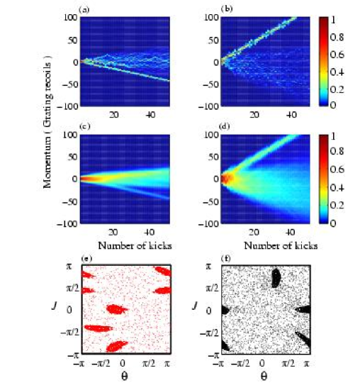
Figure 1: (Color online) Numerical simulation for the quantum accelerator modes that are produced with $g=9.81$ ms^-2, $T=132.0\mu$s. In column 1 (a, c, e), $\phi_{d}=0.8\pi$ and the $(5,2)$ quantum accelerator mode is produced; in column 2 (b, d, f), $\phi_{d}=2.4\pi$ and the $(3,1)$ quantum accelerator mode results. (a) and (b) show the momentum variation with the number of kicks for a single initial plane wave with $\beta=0$, (c) and (d) show the evolution of an atomic cloud with initial temperature $5\mu$K, and (e) and (f) show stroboscopic Poincaré sections determined by Eq. (2), with $T=132.0\mu$s ($\epsilon=-0.135$). The colorbar indicates the population, in arbitrary units.

We first examine the high-order quantum accelerator mode close to the Talbot time, $T_{\mbox{\scriptsize T}}=133.4\mu$s, for the case of a single initial quasimomentum state. We take the value $\beta=0$, and consider the case where $T=132.0\mu$s and the local gravity value $g=9.81$ ms^-2. We apply two different kicking strengths to the atoms, $\phi_{d}=0.8\pi$ and $2.4\pi$. The results of our numerical simulations, shown in Figs. 1(a) and 1(b), demonstrate that atoms evolving under $\phi_{d}=0.8\pi$ undergo a negative momentum transfer, while the atoms experiencing $\phi_{d}=2.4\pi$ undergo a positive momentum transfer. The phase maps given in Figs. 1(e) and 1(f), along with Eq. (3), show that for the lower kicking strength the quantum accelerator mode is $(5,2)$, while for the higher kicking strength the quantum accelerator mode is $(3,1)$.

Within a given quasimomentum subspace, the values of $J$ available for the initial state are equal to $(k+\beta)|\epsilon|$, where $k$ is an integer. In the case of a narrow initial momentum distribution, we expect the value of $\beta$, offsetting the available momentum spectrum, to affect the significance of that subspace’s contribution to a physically observable quantum accelerator mode. Such an effect is clearly of decreasing relevance as $\epsilon$ vanishes Fishman2002 ; Bach2005 . This general observation is borne out by numerical simulation.

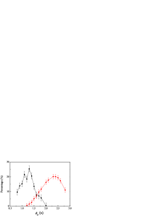
Figure 2: (Color online) Variation of the percentage of atoms in the $(5,2)$ and $(3,1)$ quantum accelerator modes as $\phi_{d}$ changes. The atomic ensemble is prepared at $5\mu$K, and $T=132.0\mu$s. The $(5,2)$ mode (squares) appears with lower kicking strength, and $(3,1)$ mode (circles) appears when the kicking strength increases. The error bar illustrates the typical spread of population in a specific quantum accelerator mode obtained from the simulation.

For the case of a thermal atomic cloud, such as the $1\times 10^{7}$ atoms at $5\mu$K with a Gaussian initial momentum distribution in which all $\beta$ are populated more-or-less equally, as used in our experiments, the dependence of the acceleration on the kicking strength is shown in Figs. 1(c) and 1(d). As expected, the $(5,2)$ and $(3,1)$ quantum accelerator modes, respectively, are produced. For this system, we can ask at which kicking strength the different quantum accelerator modes appear. The variation of the population in each quantum accelerator mode as a function of $\phi_{d}$, deduced from the numerical simulations, is shown in Fig. 2. When the kicking strength is less than $1.2\pi$, the atoms occupy the $(5,2)$ mode and the $(3,1)$ mode is absent. As one increases the kicking strength, the $(5,2)$ mode gradually disappears while the $(3,1)$ mode comes to dominate; on further increasing $\phi_{d}$, the $(5,2)$ mode dies completely. There is a range of $\phi_{d}$, centered on the value $1.6\pi$, where the quantum accelerator modes co-exist and atoms can be accelerated in two different modes simultaneously, with different directions of momentum transfer.

II.5 Tuning the effective gravitational acceleration

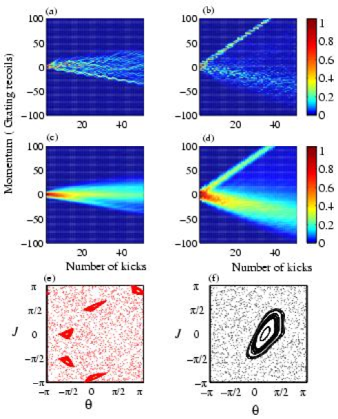
Figure 3: (Color online) Numerical simulation for the quantum accelerator modes that are produced with $g=20.10$ ms^-2, $T=137.0\mu$s. In column 1 (a, c, e), $\phi_{d}=0.8\pi$ and the $(5,-4)$ quantum accelerator mode is produced; in column 2 (b, d, e), $\phi_{d}=2.4\pi$ and the $(1,-1)$ (b, d, f) quantum accelerator mode results. (a) and (b) show the momentum variation with the number of kicks for a single initial plane wave with $\beta=0$, (c) and (d) show the evolution of an atomic cloud with initial temperature $5\mu$K, and (e) and (f) show stroboscopic Poincaré sections determined by Eq. (2), with $T=137.0\mu$s ($\epsilon=0.336$). The colorbar indicates the population, in arbitrary units.

It is possible to vary the value of the effective gravitational acceleration applied to the atoms in our experiment, and hence $\Omega$. This is accomplished by using an electro-optic modulator to vary the phase difference between the down-going and retro-reflected beams, and hence to move the profile of the standing wave dArcy2001 ; Ma2004 . This allows us to reach other parameter combinations that yield simultaneous acceleration in different directions. For example, if we tune the effective gravity to $20.10$ ms^-2 and choose a kicking period of $T=137.0\mu$s, the occupied quantum accelerator mode is $(5,-4)$ for the atoms which experience $\phi_{d}=0.8\pi$ and $(1,-1)$ for those which evolve under $\phi_{d}=2.4\pi$. The results of the corresponding numerical simulations are shown in Fig. 3.

Hence the momentum transferred by each kick can be varied by properly selecting the effective gravitational acceleration, kicking period and kicking strength in order to single out particular quantum accelerator modes. We have also found a large number of other conditions where atoms are accelerated in different quantum accelerator modes, according to the value of $\phi_{d}$.

III Incorporation of electronic degrees of freedom

III.1 Using an electronic superposition state

Within a given parameter regime, i.e., for particular values of $\phi_{d}$ and $g$, and restricting ourselves to a single plane-wave as the initial condition, it is not possible to optimally occupy two quantum accelerator modes for simultaneous acceleration. This can be understood by realizing that coexisting quantum accelerator modes must necessarily occupy different regions of pseudoclassical phase space.

An efficient way to obtain simultaneous momentum transfer in two directions is to start with a coherent superposition of internal atomic states so as to optimally change $\phi_{d}$ separately. These internal states, produced using a microwave pulse, experience different kicking strengths. This allows us to have a situation where the same initial motional state experiences two different two different kicking strengths, and maximally occupies two different quantum accelerator modes, resulting in different momentum transfers to the two parts of the superposition.

Considering two general electronic states $|a\rangle$ and $|b\rangle$, the desired model Hamiltonian has the form Schlunk2003a

$$\hat{H}_{ab}=\hat{H}(\phi_{d}^{a})|a\rangle\langle a|+\hat{H}(\phi_{d}^{b})|b\rangle\langle b|+\frac{\hbar\omega_{ab}}{2}(|b\rangle\langle b|-|a\rangle\langle a|),$$ (4)

where $\hbar\omega_{ab}$ is the energy gap between $|a\rangle$ and $|b\rangle$, and $\hat{H}(\phi_{d}^{a})$ and $\hat{H}(\phi_{d}^{b})$ are equal to the atomic center of mass Hamiltonian of Eq. (1), with $\phi_{d}=\phi_{d}^{a}$ and $\phi_{d}^{b}$, respectively. In our experiments, $|a\rangle$ may correspond the $|F=3,m_{F}=0\rangle$ substate of the ground state of cesium, and $|b\rangle$ may correspond to the $|F=4,m_{F}=0\rangle$ substate; henceforth these substates will be denoted $|a\rangle$ and $|b\rangle$, respectively.

III.2 Use of microwave pulses for state preparation

The population of cesium atoms in the states $|a\rangle$ and $|b\rangle$ can be modified by a $9.18$ GHz microwave pulse, resonant with the $|b\rangle\rightarrow|a\rangle$ hyperfine transition Schlunk2003a . The $9.18$ GHz difference between the transition frequencies from the states $|a\rangle$ and $|b\rangle$ to any given excited state means that atoms in the two internal states will experience different values of $\phi_{d}$ when exposed to laser light of a particular intensity and detuning.

A coherent superposition of $|a\rangle$ and $|b\rangle$ can be achieved experimentally by applying a $\pi/2$ microwave pulse to a sample of atoms in state $|b\rangle$, in which they are trapped and cooled. The intensity and detuning of the light creating the kicking potential can be selected so as to apply the correct values of $\phi_{d}$ to the states $|a\rangle$ and $|b\rangle$ to permit efficient population of the required quantum accelerator modes. For example, with our current experimental setup, it is feasible to have a value $\phi_{d}=0.8\pi$ for state $|a\rangle$, while the corresponding value for state $|b\rangle$ is $\phi_{d}=2.4\pi$. Without any alteration to the effective value of $g$, atoms in $|b\rangle$ state will be kicked in one direction [in the $(3,1)$ quantum accelerator mode] while atoms in $|a\rangle$ state will be kicked in the other [in the $(5,2)$ quantum accelerator mode], as shown in Fig.1. The transfer of momentum is therefore dependent on the internal state, which is just what one needs for a beam splitter. This may well lead to a new type of interferometry based on this beam splitting mechanism and will be the subject of future investigations.

III.3 State-dependent evolution

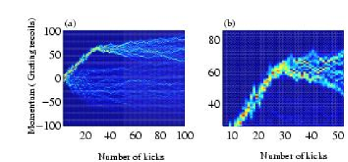
Figure 4: (Color online)(a) Momentum variation with number of kicks, for $\beta=0$, $\phi_{d}=2.2\pi$ for state $|a\rangle$ and $\phi_{d}=0.7\pi$ for state $|b\rangle$, with $T=132.0\mu$s and $g=9.81$ ms^-2. A state-flipping microwave pulse is applied after the $25$th kick. The zoom-in around the switch point is shown in (b).

In this paper, however, we are focusing on the application of the technique of simultaneous momentum transfer that quantum accelerator modes provide to quantum random walks. The state-dependence of the momentum transfer permits the state-dependent evolution required for a quantum, rather than classical, random walk. With atoms initially in a superposition of the $|a\rangle$ and $|b\rangle$ states, we can apply kicks to accelerate the atoms in the two states in different directions.

To investigate how the methods of manipulating the internal state of the atoms permit momentum control, we numerically simulate a sequence in which we accelerate atoms in state $|b\rangle$ for $25$ kicks with $\phi_{d}=2.2\pi$, and we then apply a $\pi$ microwave pulse to pump all atoms from state $|b\rangle$ into state $|a\rangle$, for which $\phi_{d}=0.7\pi$. $T=132.0\mu$s and $g=9.81$ ms^-2 are kept constant during the process. The results of the simulation are shown in Fig. 4. After the switch, atoms in $|b\rangle$ cease increasing momentum in their original direction and about $30$% of them begin to accumulate momentum in the opposite direction, corresponding to the quantum accelerator mode with the lower kicking strength. Optimization of the efficiency of transfer from one quantum accelerator mode to the other needs a more detailed investigation, as we now discuss.

III.4 Optimizing the switch property

An ideal switch between different momentum transfer modes requires the wavefunction of one quantum accelerator mode to have an overlap with the other mode at the time of switching. From the FGR analysis, this implies that better switching efficiency will occur when the stable islands in pseudoclassical phase space for the two quantum accelerator modes overlap Buchleitner2005 .

This is illustrated in Fig. 5, where $g=7.26$ ms^-2, $T=131.0\mu$s, $\phi_{d}=0.6\pi$ and $3.8\pi$ for two different states. The overlap between the stable islands for the lower kicking strength [mode $(1,0)$, blue dots] and the higher kicking strength [mode $(4,1)$, red dots] in Fig. 5(a) is greater than that in Figs. 1(e) and 1(f), or Figs. 3(e) and 3(f). This, as we would expect, leads to a more efficient transfer of population between the quantum accelerator modes when the atomic internal state is flipped by a microwave pulse, as shown by the comparison between Fig. 5(b) and Fig. 4(b). About $80$% of the atoms are successfully transferred from one mode to the other.

The $\epsilon$-classical map thus provides the capability of using the overlap criterion to search in parameter space to find the best switching condition. A complete search of the relevant phase space is a substantial enterprise, and will be part of a longer term effort to optimize the operation of a practical random-walker.

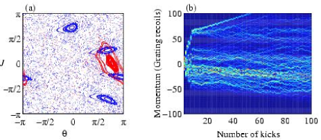
Figure 5: (Color online) (a) Phase map of quantum accelerator modes, with $\beta=0.1$, $T=131.0\mu$s, $g=7.26$ ms^-2, $\phi_{d}=3.8\pi$ for state $|a\rangle$ (red dots, ) and $\phi_{d}=0.6\pi$ for state $|b\rangle$ (blue dots). (b) Momentum variation with number of kicks; a state-flipping $\pi$ pulse occurs after the $8$th kick.

IV Near-ideal biased quantum random walk

We now turn to the implementation of a quantum random walk using the state-dependent acceleration process we have just described. Applying a $\pi/2$ microwave pulse after each kick is equivalent to the “coin-flipping” process introduced by Aharanov in his discussion of a quantum random walk Aharanov1993 . In this section, we would like to show how we could use quantum accelerator modes to implement a quantum random walk.

This scheme also introduces different features from the Aharanov model, and we therefore name this model a “biased” quantum random walk in momentum space. In a biased quantum walk, the “coined” state, which determines the direction atoms move in by the extra degree of freedom of “sides” (discussed in Ref. Aharanov1993 ), is the pair of hyperfine states of the atoms and the momentum transfer per step, i.e., the walk speed, is determined by the order of quantum accelerator modes. This can be altered [see Eq. (3)] by selecting different values of the parameters $K$ and $\Omega$ that determine the acceleration. In this way atoms can be made to perform a Hadamard-style quantum random walk in momentum space.

It is important to note that atoms are divided to three different classes in the case of quantum accelerator modes considered here: two of them fall into two different accelerator modes, thus obtaining different momentum changes in each step, and the rest of the atoms are “left behind”. There is an overall recoil in the opposite direction to the quantum accelerator modes NoteRecoil , but within this the motion is diffusive rather than the coherent motion of quantum accelerator modes. In order to understand better how such a system could be used to realise a quantum random walk we propose the following simplified model. Our model is a “biased quantum random walk” for our coined quantum accelerator mode, where atoms not only walk in two different directions, but can be left behind.

The walk operator $S$ then reads,

$$\begin{split}S=&(1-\gamma)(|a\rangle\langle a|\otimes\sum_{i}|i-\delta_{1}\rangle\langle i|\\ &+|b\rangle\langle b|\otimes\sum_{i}|i+\delta_{2}\rangle\langle i|)+\gamma\sum_{i}|i\rangle\langle i|,\end{split}$$ (5)

where integers $i$ indicate the momentum states, and $\delta_{1}$ and $\delta_{2}$ corresponding to selected accelerator modes of $(\mathfrak{p}_{1},\mathfrak{j}_{1})$ and $(\mathfrak{p}_{2},\mathfrak{j}_{2})$. Here $\gamma$ is the “leaving behind” amplitude.

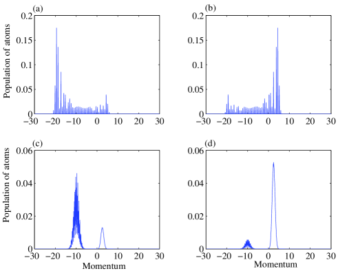
Figure 6: The momentum distribution (in arbitrary units) of the biased quantum random walk with a Hadamard coin after 50 steps, starting in state $|a\rangle\otimes|0\rangle$ for (a) and (c), and state $|b\rangle\otimes|0\rangle$ for (b) and (d). The parameter $\gamma$, defined in Eq. 5, is $0$ for (a, b) and $0.5$ for (c, d). The momentum increase is $0.25$ units per step to the negative direction and $0.1$ units per step to the positive direction.

The results of the numerical simulation of this biased quantum random walk are shown in Fig. 6. Quantum accelerator modes increase the momentum of a group of atoms linearly with the number of kicks, and this means that the effective “diffusion” of the biased walk will also be linearly proportional to the number of kicks, or “superdiffusive.” We should expect atoms moving faster in one direction than the other due to the difference in the walking speeds of the two occupied quantum accelerator modes. Walks with non-zero values of the parameter $\gamma$ have very different distributions from those with $\gamma=0$. In particular walks with $\gamma\neq 0$ will fill up the momentum gaps produced by a “pure” $\gamma=0$ quantum random walk.

From Fig. 5 about $80$% of atoms have a good switch from one mode to another and $20$% are left behind, for appropriate values of $\beta$, $g$, and $\phi_{d}$. In this way, atoms could perform quantum random walk for several steps. A future study to perfect the switching property is necessary. The value of such walks in search algorithms, and ways of varying $\gamma$, will be the subject of future work. In this paper we simply want to emphasis the potential interest and value of state-dependent momentum transfer in quantum accelerator modes, of the type we investigate here.

V Conclusions

In conclusion, we have described a novel way to produce state-dependent momentum transfer in a group of atoms. We believe that this offers a new route to produce quantum random walks in the laboratory with feasible experimental parameters. In particular, the next generation of experiments with enhanced velocity selection will put practical realizations well within reach. The state-dependent walk controlled through the parameters of the external perturbation is worthy of investigation in its own right. There are three independent control parameters in the basic $\delta$-kicked accelerator, namely the driving strength, the effective gravitational acceleration, and the value of the commutator $|\epsilon|$. In an atom-optical configuration these can all be tuned independently. There are thus many parameter regimes available particularly when considering the additional degrees of freedom offered by superposition states. The full range of such phenomena, and their relevance to quantum random walks, quantum resonances and quantum chaos in superposition states, awaits exploration.

References

- (1) M. K. Oberthaler, R. M. Godun, M. B. d’Arcy, G. S. Summy, and K. Burnett, Phys. Rev. Lett. 83, 4447 (1999).
- (2) R. M. Godun, M. B. d’Arcy, M. K. Oberthaler, G. S. Summy, and K. Burnett, Phys. Rev. A 62, 013411 (2000).
- (3) M. B. d’Arcy, R. M. Godun, M. K. Oberthaler, G. S. Summy, K. Burnett, and S. A. Gardiner, Phys. Rev. E 64, 056233 (2001).
- (4) S. Fishman, I. Guarneri, and L. Rebuzzini, Phys. Rev. Lett. 89, 084101 (2002); J. Stat. Phys. 110, 911 (2003).
- (5) R. Bach, K. Burnett, M. B. d’Arcy, and S. A. Gardiner, Phys. Rev. A 71, 033417 (2005).
- (6) S. Schlunk, M. B. d’Arcy, S. A. Gardiner, and G. S. Summy, Phys. Rev. Lett. 90, 124102 (2003).
- (7) S. Schlunk, M. B. d’Arcy, S. A. Gardiner, D. Cassettari, R. M. Godun, and G. S. Summy, Phys. Rev. Lett. 90, 054101 (2003).
- (8) Z.-Y. Ma, M. B. d’Arcy, and S. A. Gardiner, Phys. Rev. Lett. 93, 164101 (2004).
- (9) A. Buchleitner, M. B. d’Arcy, S. Fishman, S. A. Gardiner, I. Guarneri, Z.-Y. Ma, L. Rebuzzini, and G. S. Summy, e-print physics/0501146.
- (10) Y. Aharonov, L. Davidovich, and N. Zagury, Phys. Rev. A, 48, 1687 (1993).
- (11) E. Bach, S. Coppersmith, M. P. Goldschen, R. Joynt, and J. Watrous, J. Comput. Syst. Sci. 69, 562 (2004); J. Kempe, Contemporary Physics, 44 307 (2003); Y. Omar, N. Paunkovic, L. Sheridan, and S. Bose, quant-ph/0411065; P. L. Knight, E. Roldan, and J. E. Sipe, J. Mod. Optic. 51, 1761 (2004).
- (12) O. Buerschaper and K. Burnett, quant-ph/0406039; A. Romanelli, A. Auyuanet, R. Siri, G. Abal, and R. Donangelo, Physica A 352, 409 (2005); A. Wojcik, T. Luczak, P. Kurzynski, A. Grudka, and M. Bednarska, Phys. Rev. Lett. 93, 180601 (2004).
- (13) B. C. Travaglione and G. J. Milburn, Phys. Rev. A 65, 032310 (2002).
- (14) B. C. Sanders, S. D. Bartlett, B. Tregenna, and P. L. Knight, Phys. Rev. A 67, 042305 (2003); P. L. Knight, E. Roldan, and J. E. Sipe, Opt. Commun. 227, 147 (2003); E. Roldan and J.C. Soriano, quant-ph/0503069.
- (15) W. Dür, R. Raussendorf, V. M. Kendon, and H.-J. Briegel, Phys. Rev. A 66 052319 (2002).
- (16) F. L. Moore, J. C. Robinson, C. F. Bharucha, B. Sundaram, and M. G. Raizen, Phys. Rev. Lett. 75, 4598 (1995); J. C. Robinson, C. F. Bharucha, K. W. Madison, F. L. Moore, B. Sundaram, S. R. Wilkinson, and M. G. Raizen, ibid. 76, 3304 (1996); D. A. Steck, V. Milner, W. H. Oskay, and M. G. Raizen, Phys. Rev. E 62, 3461 (2000); W. H. Oskay, D. A. Steck, and M. G. Raizen, Chaos, Solitons & Fractals 16, 409 (2003); W. H. Oskay, D. A. Steck, V. Milner, B. G. Klappauf, and M. G. Raizen, Opt. Comm. 179, 137 (2000); B. G. Klappauf, W. H. Oskay, D. A. Steck, and M. G. Raizen, Phys. Rev. Lett. 81, 4044 (1998); B. G. Klappauf, W. H. Oskay, D. A. Steck, and M. G. Raizen, Physica D 131, 78 (1999); V. Milner, D. A. Steck, W. H. Oskay, and M. G. Raizen, Phys. Rev. E 61, 7223 (2000); C. F. Bharucha, J. C. Robinson, F. L. Moore, B. Sundaram, Q. Niu, and M. G. Raizen, Phys. Rev. E 60, 3881 (1999).
- (17) H. Ammann, R. Gray, I. Shvarchuk, and N. Christensen, Phys. Rev. Lett. 80, 4111 (1998); H. Ammann and N. Christensen, Phys. Rev. E 57, 354 (1998); K. Vant, G. Ball, H. Ammann, and N. Christensen, ibid. 59, 2846 (1999); K. Vant, G. Ball, and N. Christensen, ibid. 61, 5994 (2000); M. Sadgrove, A. Hilliard, T. Mullins, S. Parkins, and R. Leonhardt, ibid. 70, 036217 (2004); A. C. Doherty, K. M. D. Vant, G. H. Ball, N. Christensen, and R. Leonhardt, J. Opt. B 2, 605 (2000); M. E. K. Williams, M. P. Sadgrove, A. J. Daley, R. N. C. Gray, S. M. Tan, A. S. Parkins, N. Christensen, and R. Leonhardt ibid. 6, 28 (2004).
- (18) P. Szriftgiser, J. Ringot, D. Delande, and J. C. Garreau, Phys. Rev. Lett. 89, 224101 (2002).
- (19) G. Duffy, S. Parkins, T. Müller, M. Sadgrove, R. Leonhardt, and A. C. Wilson, Phys. Rev. E 70, 056206 (2004).
- (20) P. H. Jones, M. M. Stocklin, G. Hur, and T. S. Monteiro, Phys. Rev. Lett. 93, 223002 (2004); P. H. Jones, M. Goonasakera, H. E. Saunders-Singer, and D. R. Meacher, Europhys. Lett. 67, 928 (2004).
- (21) C. Ryu, M. Andersen, A. Vaziri, M. B. d’Arcy, J. M. Grossman, K. Helmerson, and W. D. Phillips, in preparation (2005).
- (22) J. W. Goodman, Introduction to Fourier Optics (McGraw-Hill, New York, 1996).
- (23) N. W. Ashcroft and N. D. Mermin, Solid State Physics (Saundeers College Publishing, Fort Worth, 1976).
- (24) S. A. Gardiner, J. I. Cirac, and P. Zoller, Phys. Rev. Lett. 79, 4790 (1997).
- (25) If all possible initial conditions are populated, i.e., the initial distribution of atoms is large enough to cover several phase-space cells, then in the freely-falling frame the average momentum is conserved. Thus, the unaccelerated cloud always on average “recoils” from the quantum accelerator modes.