A conjecture for turbulent flow

Abstract

In this paper, basing on a generalized Newtonian dynamics (GND) approach which has been proposed elsewhere we present a conjecture for turbulent flow. We firstly utilize the GND to reasonably unify the two phenomenological methods recently proposed of the water movement in unsaturated soils. Then in the same way a modified Euler equation (MEE) is yielded. Under a zero-order approximation, a simple split solution of the MEE can be obtained that shows flow fluids would have a velocity field with the power-law scaling feature (power-law fluid) for the case of high Reynolds number.

Turbulent flow is one of the most bewildering phenomena in nature. Ever since a hundred years, people have initiated many theories to explain it. These theories give different phenomenological descriptions, and some of them are in good agreement with experimental data and provide some very useful clues for our understanding of true essence of turbulent flow. However, up to now, we can not employ a unified framework to describe turbulent flow yet, not to mention explaining it. we even can not give a good definition of turbulence so that we can quantitatively determine whether turbulent flow has appeared in a fluid.

In this paper, we would present a conjecture for turbulent flow with the generalized Newtonian dynamics (GND) in order to better describe turbulence.

The GND describes the fractal world by means of a fractional dimensional kinetic velocity (or mass). In the anomalous displacement variation model (ADVM), its one-dimensional basic dynamics equation in terms of the Newtonian kinematics equation form can be written as follows:

$$m\ddot{x}=\alpha(\sum_{i}F_{i})|x|^{1-q}+\kappa\frac{(\dot{x})^{2}}{x}.$$ (1)

Here $m$ is mass of a particle, $F_{i}$ is the i-th external force acting on the particle, $q$ is a velocity fractal index (vfi) and $\dot{x}$ denotes $dx/dt$. The right-hand side of the generalized Newtonian dynamics equation (1) can be understood as the effective forces acting on the particle in the Euclidean space of the fractal environment, and the two constants, $\alpha$ and $\kappa$, which are given by $\alpha=m/(qm_{q})$ and $\kappa=m(1-q)$ respectively, are the effective force coefficients. Here $m_{q}$ is an effective mass of the particle in the fractal environment, which has a dimension of $[kg\cdot m^{1-q}]$. The generalized Newtonian dynamics Eq. (1) can be reduced to the Newtonian kinematics equation $m\ddot{x}=\sum_{i}F_{i}$ when $q=1$ namely the fractal velocity $\pm\frac{d|x|^{q}}{dt}$ becomes the ordinary velocity $\frac{dx}{dt}$.

It is seen that the term $\kappa\frac{(\dot{x})^{2}}{x}$ in Eq. (1) is an additional force which can be eliminated only when the fractal environment around the particle disappears, namely $q=1$. We call the term $\kappa\frac{(\dot{x})^{2}}{x}$ the fractal force (FF). The FF appears in the complex fractal environment, its additional property is similar to that of Coriolis force in a rotational inertial system, but the origin or the practicable situation of it is still unknown for us.

The cascade process in turbulence shows turbulent flow is a type of the fractal phenomenon. Particularly scaling law discovered by Kolmogorov and the characteristic of the $\frac{1}{f}$ power spectrum of turbulence signal can also evidently exhibit that. Here we would assume all kinds of turbulent flow as well as process from laminar flow or convection to turbulence can be described on basis of the fractal geometry. The fractal geometry, whose detail contents can be reviewed in Ref. , was initialized by Mandelbrot.

Accordingly, we want to introduce the GND into turbulence. We have a definition of fractal velocity according to the anomalous displacement variation model (ADVM):

$$v_{q}=\frac{dx^{\prime}}{dt}=\pm\frac{d|x|^{q}}{dt}=q|x|^{q-1}\frac{dx}{dt}$$ (2)

where $q$ is the velocity fractal index (vfi). We assume a particle needs a $n\Delta t$ time length to “jump” a $(n\Delta x)^{q}$ displacement length, then the instantaneous motion state of the particle can be expressed by Eq. (2). Here $\Delta x$ and $\Delta t$ is a fixed displacement length and time interval respectively, and $n$ is a natural number representing the $n$-th step of the particle. Because the instantaneous velocity of the particle can be written as

$$\ \ v_{n}=\lim_{\Delta t\to 0}\frac{(n\Delta x)^{q}-[(n-1)\Delta x]^{q}}{\Delta t}$$ (3)

$$=\lim_{\Delta t\to 0}\frac{(n\Delta x)^{q}-[(n-1)\Delta x]^{q}}{\Delta x}\frac{\Delta x}{\Delta t}\ \ \ ;$$ (4)

we let $\Delta x$=$\Delta|x(t)|$, $n\Delta x$=$|x(t)|$, and both $\Delta|x(t)|$ and $\Delta t$ be an arbitrary small increment; allowing for the directivity of velocity, Eq. (4) thus can be rewritten with $x=\pm|x|$ as Eq. (2) where $x^{\prime}=\pm|x|^{q}$ which represents the particle’s displacement in the complex environment (which is somewhat different from real physical displacement). Similarly, we have another form of definition of fractal velocity according to the anomalous time variation model (ATVM):

$$v^{\prime}_{q}=\frac{dx}{dt^{\prime}}=\frac{dx}{dt^{q}}=\frac{1}{q}t^{1-q}\frac{dx}{dt}$$ (5)

In Fig. 1, we give a schematic description of the two models.

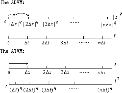
Figure 1: Schematic representation of the anomalous displacement variation model (ADVM) and the anomalous time variation model (ATVM) of anomalous motion. In the ADVM, the particle takes the $n\Delta t$ time length to anomalously move (generally jump) the $(n\Delta x)^{q}$ displacement length along the x-axis. In the ATVM, the particle needs the $(n\Delta t)^{q}$ time length to anomalously walk (generally run and wait) the $n\Delta x$ displacement length along the x-axis.

But, in fact, Eq. (2) and Eq. (5) are only different descriptions of the same physical fact. For example, the fact that a particle walks the $(n\Delta x)^{q}$ displacement length within the $n\Delta t$ time interval can also be stated in another word that the particle needs $(n\Delta t)^{p}$ time interval to walk $n\Delta x$ displacement length $(p\neq q)$. In addition, $\lambda^{1-q}x^{\prime}$ and $t$ are real physical variables in Eq. (2) while $x$ is only a scaling variable, where $\lambda$ denotes a characteristic length and $m\lambda^{1-q}=m_{q}$; similarly $x$ and $\tau^{1-q}t^{\prime}$ in Eq. (5) are real physical variables while $t$ is only a scaling variable, where $\tau$ is a characteristic time and $m\tau^{2q-2}=m^{\prime}_{q}$. Note that $x-$space is changed to $x^{q}-$space when a particle is moving with time, namely ordinary scaling matching structure of time and space is modified, but any force (except those related to velocity) is invariant from the ordinary environment to the fractal space.

With the help of the GND approach, we can easily unify the two phenomenological methods recently proposed of the water percolation in unsaturated soils. In the unsaturated soil-water transport, the water flux for the horizontal one-dimensional column case follows the Buckingham-Darcy law:

$$Q=-k(\theta)\frac{\partial\psi}{\partial x}$$ (6)

where $Q$ denotes the volume flow rate per unit area, $k$ is unsaturated hydraulic conductivity, $\psi$ is the hydraulic pressure head and $\theta$ is the soil water content; and the customary Richards’ equation

$$\frac{\partial\theta}{\partial t}=\frac{\partial}{\partial x}[D(\theta)\frac{\partial\theta}{\partial x}]$$ (7)

can be arrived at by combining Eq. (6) and the mass conservation equation $\frac{\partial\theta}{\partial t}+\frac{\partial Q}{\partial x}=0$ with $D(\theta)=k(\theta)\frac{d\psi}{d\theta}$. Here $D(\theta)$ is the soil water diffusivity.

It is necessary to emphasize that movement of liquid water in soils is not a diffusion phenomenon . Conversely, it is a kind of macroscopic flow motion which is based on Navier-Stokes law. Phillip derived the conclusion that Buckingham-Darcy law follows from the Navier-Stokes equation with $(\vec{u}\cdot\nabla)\vec{u}\simeq 0$: $v_{k}\nabla^{2}\vec{u}=\nabla\phi$ where $v_{k}$ is dynamical viscosity and $\phi$ is total potential . Here no concept of probability appears.

However, deviations from Eq. (7) cause further assumptions that the diffusivity has a dependence on distance given by $|x|^{-\beta}D(\theta)$ or the diffusivity is a time-dependent quantity given by $t^{2m-1}D(\theta)$ . Here $m$ is a positive constant. We now want to unify the above two assumptions and do not need to introduce other models for microscopic anomalous transport.

In the GND framework, the reduced Navier-Stokes equation is rewritten as $v^{\prime}_{k}\nabla^{2}\vec{u}_{s}=\nabla\phi$ where $\vec{u}_{s}$ is fractal velocity. Then the Richards’ equation is generalized as

$$\frac{\partial\theta}{\partial t}=\frac{1}{s}\frac{\partial}{\partial x}(|x|^{1-s}D_{s}(\theta)\frac{\partial\theta}{\partial x})$$ (8)

and

$$\frac{\partial\theta}{\partial t}=s\frac{\partial}{\partial x}(t^{s-1}D_{s}(\theta)\frac{\partial\theta}{\partial x})\ ,$$ (9)

respectively. Here $s$ is the vfi and $D_{s}(\theta)$ is a fractal soil water diffusivity.

Eq. (8) and Eq. (9) are similar to the generalized Richards’ equations proposed in [9] and [10], respectively, which have been shown to be valid for some experiment data. But we can unify the two kinds of assumption in one framework, and it seems more reasonable because previous frameworks of anomalous diffusion are not appropriated for describing essentially macroscopic flow movements.

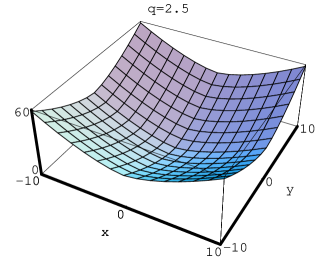
Figure 2: Velocity field $v_{x}(x,y)$ given by a solution of the MEE Eq. (19) for different values of $q$. The solution reflects motion state of a flow in the fractal environment. Here $a$ and $b$ are both taken 1.

For the turbulence problem, we can obtain a modified Euler equation (MEE) from the GNKE Eq. (1) according to the principle of the GND:

$$\frac{\partial\vec{v}}{\partial t}+(\vec{v}\cdot\nabla)\vec{v}=-\frac{\alpha}{\rho}\nabla_{q}p+\frac{\alpha}{\rho}\vec{F}_{q}+\beta\vec{a}_{f}$$ (10)

where $\alpha=\frac{m}{qm_{q}}$, $\beta=1-q$,

$$\nabla_{q}=\begin{pmatrix}|x|^{1-q}\frac{\partial}{\partial x}\\ |y|^{1-q}\frac{\partial}{\partial y}\\ |z|^{1-q}\frac{\partial}{\partial z}\end{pmatrix}\ \ ,$$ (11)

$$\vec{F_{q}}=\begin{pmatrix}|x|^{1-q}\frac{dF_{x}}{dV}\\ |y|^{1-q}\frac{dF_{y}}{dV}\\ |z|^{1-q}\frac{dF_{z}}{dV}\end{pmatrix}\ \ ,$$ (12)

$$\vec{a_{f}}=\begin{pmatrix}\frac{(\dot{x})^{2}}{x}\\ \frac{(\dot{y})^{2}}{y}\\ \frac{(\dot{z})^{2}}{z}\end{pmatrix}\ \ ,$$ (13)

$\rho$ is density of a fluid; $-\alpha dV\nabla_{q}p$ is an effective pressure acting on certain a volume element $dV$ from surrounding fluid bodies and $\vec{F}_{q}$ is considered as an effective complex force field acting on a volume element $dV$ of the fluid where $dF_{i}$ $(i=x,y,z)$ is a real physical force (other than pressure) acting on a volume element $dV$. We notice that $\vec{a}_{f}$ has the same dimension as another nonlinear term $(\vec{v}\cdot\nabla)\vec{v}$.

We call $\nabla_{q}$ the fractional gradient operator, and also we notice that $\rho\beta\vec{a_{f}}$ is exactly the fractal force on a unit volume of fluid. In addition, the coefficient $\alpha$ with the dimension [$m^{q-1}$] can be seen as $\lambda^{q-1}$. Here $\lambda$ is a characteristic length of the fluid. We see the MEE (10) will will recover the ordinary Euler equation:

$$\frac{\partial\vec{v}}{\partial t}+(\vec{v}\cdot\nabla)\vec{v}=-\frac{1}{\rho}\nabla p+\frac{1}{\rho}\frac{d\vec{F}}{dV}\ .$$ (14)

Here $d\vec{F}$ is force (other than pressure) acting on the volume element $dV$.

The MEE reflects the situation of a fluid with fractal feature, since it is derived directly from a fractal velocity which describes the fractal state of a system. We think the ordinary Euler equation can not play a role in determining the fractal state of the fluid, for the nonlinear term $(\vec{v}\cdot\nabla)\vec{v}$ is only a kinematic factor rather than a dynamical factor like the term $(1-q)\vec{a}_{f}$ in the MEE. In other words, when the fluid becomes in a fractal state, the fluid would be acted on by a special fractal force which appears only in the fractal situation, and the fractal force can also be seen as an external energy input; at the same time, ordinary forces will also be deformed, but these changes can not follow naturally from the ordinary Euler equation. Of course, the process from a laminar flow or a convection current to turbulent flow is controlled by real physical parameters such as velocity of the fluid or temperature difference, these parameters often can be combined into a dimensionless number such as the Reynolds number $Re$. Particularly there is a critical Reynolds number $Rec$. When the Reynolds number of a fluid is above $Rec$, turbulence happens. That can make us guess that the vfi $q$ is a function of these dimensionless numbers and critical dimensionless numbers such as $Re$ and $Rec$ such that the fact that turbulence emerges when $Re>Rec$ is equal to the situation of the MEE for $q>1$ (or $q<1$).

The viscous term of a fluid can be directly added in $\vec{F_{q}}$ in Eq. (10), but here we would take a look at solutions of the MEE in a range of high Reynolds number.

We study the MEE for the case of the two-dimensional incompressible and constant flow, and we consider $\vec{F}_{q}=0$; then Eq. (10) becomes

$$\left\{\begin{array}[]{c}v_{x}|x|^{q-1}\frac{\partial v_{x}}{\partial x}+v_{y}|x|^{q-1}\frac{\partial v_{x}}{\partial y}=-\frac{\alpha}{\rho}\frac{\partial p}{\partial x}+\beta|x|^{q-1}\frac{v^{2}_{x}}{x}\\ v_{x}|y|^{q-1}\frac{\partial v_{y}}{\partial x}+v_{y}|y|^{q-1}\frac{\partial v_{y}}{\partial y}=-\frac{\alpha}{\rho}\frac{\partial p}{\partial y}+\beta|y|^{q-1}\frac{v^{2}_{y}}{y}\end{array}\right.\$$ (15)

We make such an approximation that

$$\left\{\begin{array}[]{c}a|x|^{q-1}\frac{\partial v_{x}}{\partial x}+b|x|^{q-1}\frac{\partial v_{x}}{\partial y}=-\frac{\alpha}{\rho}\frac{\partial p}{\partial x}+\beta|x|^{q-1}\frac{v^{2}_{x}}{x}\\ a|y|^{q-1}\frac{\partial v_{y}}{\partial x}+b|y|^{q-1}\frac{\partial v_{y}}{\partial y}=-\frac{\alpha}{\rho}\frac{\partial p}{\partial y}+\beta|y|^{q-1}\frac{v^{2}_{y}}{y}\end{array}\right.\$$ (16)

where $a$ and $b$, which represent the mean velocity of the fluid $\bar{v}_{x}$ and $\bar{v}_{y}$, respectively, are constant. The approximation is reasonable for a fluid with small velocity gradient.

Eliminating the pressure intensity $p$ and utilizing the continuity condition,

$$\frac{\partial v_{x}}{\partial x}+\frac{\partial v_{y}}{\partial y}=0\ ,$$ (17)

we have

$$|x|^{q-1}\frac{\partial^{2}\psi}{\partial y^{2}}+|y|^{q-1}\frac{\partial^{2}\psi}{\partial x^{2}}=\beta\frac{|x|^{q-1}}{x}\frac{\partial v^{2}_{x}}{\partial y}-\beta\frac{|y|^{q-1}}{y}\frac{\partial v^{2}_{y}}{\partial x}$$ (18)

where $\psi=bv_{x}-av_{y}$.

We let $v^{2}_{x}=\frac{(\psi+av_{y})^{2}}{b^{2}}\sim\psi^{2}$ as well as $v^{2}_{y}\sim\psi^{2}$, which is proper for a fluid whose velocity is not too large. Then we obtain a second-order partial differential equation concerning $\psi$:

$$|x|^{q-1}\frac{\partial^{2}\psi}{\partial y^{2}}+|y|^{q-1}\frac{\partial^{2}\psi}{\partial x^{2}}=\frac{\beta}{b^{2}}\frac{|x|^{q-1}}{x}\frac{\partial\psi^{2}}{\partial y}-\frac{\beta}{a^{2}}\frac{|y|^{q-1}}{y}\frac{\partial\psi^{2}}{\partial x}\ .$$ (19)

We neglect the two second partial derivative terms of $\psi$, because both of them can be seen as small quantities. Eq. (19) thus is simplified as a first-order partial differential equation:

$$b^{2}x|x|^{1-q}\frac{\partial\psi}{\partial x}=a^{2}y|y|^{1-q}\frac{\partial\psi}{\partial y}$$ (20)

whose general solution can be easily arrived at:

$$\psi=\Phi(u)=\Phi(a^{2}|x|^{q-1}+b^{2}|y|^{q-1})\ .$$ (21)

Here $\Phi$ is any continuous and differentiable function of $u$.

For simplicity, we choose $\psi$ as follows:

$$bv_{x}-av_{y}=(b-a)(a^{2}|x|^{q-1}+b^{2}|y|^{q-1})\ ,$$ (22)

such that

$$v_{x}=v_{y}=a^{2}|x|^{q-1}+b^{2}|y|^{q-1}\ .$$ (23)

Evidently, the velocity field $v_{x}$ or $v_{y}$ is a parabolic dish for different values of $q$.

Therefore, under such an approximation, we obtain a simple solution of the MEE for a two-dimensional incompressible and constant flow in the high Reynolds number limit:

$$v_{i,j}=\bar{v}_{i}^{2}|x_{i}|^{q-1}+\bar{v}_{j}^{2}|x_{j}|^{q-1}$$ (24)

where $v_{i,j}$ denotes $v_{i}$ or $v_{j}$.

We graph velocity field $v_{x}$ given by Eq. (23) for different values of $q$ in Fig. 2. Here $a$ and $b$ are both taken 1. It is clearly seen that manifold is broken when $q<1$ and the fluid velocity $v_{x}$ becomes infinity at the position $x=0$ or $y=0$. We can imagine that the fluid body could be broken up into four closed packets in each dimension if proper boundary conditions about ($x,y,v_{i,j}$) are given. Thus we can call the solution Eq. (23) for the case of $q<1$ a split solution for the MEE. The situation for $1<q<2$ is somewhat different where four convexes of the fluid are not broken. When $q>2$, velocity field of the fluid becomes an concave parabolic dish. For $q=2$ the velocity field comprises four planes and for $q=1$ a laminar flow case is recovered.

The solution reflects motion state of a flow in the fractal environment which is embodied in the MEE by both a fractal force which can be understood as an external nonlinear energy input and a fractional gradient operator $\nabla_{q}$ which is similar to the Riesz fractional derivative operator . It is important that the fractional gradient operator will simultaneously be reduced to the ordinary gradient operator when the fractal force disappears. However, whether the MEE can describe turbulent flow or not is still an open problem.

Summarizing, the fact that the GND framework can reasonably unify the two phenomenological methods recently proposed of anomalous transport of water in unsaturated soils and other satisfactory results of the GND elsewhere make us conjecture that the GND constitutes a dynamical basis of the problem of turbulence, thus a modified Euler equation (MEE) is yielded. Under a zero-order approximation, a simple split solution of the MEE can be obtained, and we see that turbulent flow would have a velocity field with the power-law scaling feature for the case of high Reynolds number.