Multifractal Detrended Fluctuation Analysis of Sunspot Time Series

Abstract

We use multifractal detrended fluctuation analysis (MF-DFA), to See query 1 study sunspot number fluctuations. The result of the MF-DFA shows that there are three crossover timescales in the fluctuation function. We discuss how the existence of the crossover timescales is related to a sinusoidal trend. Using Fourier detrended fluctuation analysis, the sinusoidal trend is eliminated. The Hurst exponent of the time series without the sinusoidal trend is $0.12\pm 0.01$. Also we find that these fluctuations have multifractal nature. Comparing the MF-DFA results for the remaining data set to those for shuffled and surrogate series, we conclude that its multifractal nature is almost entirely due to long range correlations.
Keyboard: New applications of statistical mechanics

]

I Introduction

The important feature of the sun‘s outer regions is the existence of a reasonably strong magnetic field. To the lowest order of approximation, the sun’s magnetic field is dipolar in character and is axisymmetric. The strength of the field on a typical point on the solar surface is approximately a few Gauss. There is, however significant variation in this value and there are localized regions (called $sunspots$) in which the filed can be much higher [1]. Because of the symmetry of the twisted magnetic lines as the origin of sunspots, they are generally seen in pairs or in groups of pairs at both sides of the solar equator. As the sunspot cycle progresses, spots appear closer to the sun’s equator giving rise to the so called “butterfly diagram” in the time latitude distribution [2]. The twisted magnetic field above sunspots are sites where solar flares are observed. It has been found that chromospheric flares show a very close statistical relationship with sunspots [1]. The number of sunspots is continuously changing in time in a random fashion and constitutes a typically random time series. Figure 1 shows the monthly measured number of sunspots in terms of time. The data belongs to a data set collected by the Sunspot Index Data Center (SIDC) from 1749 up to now [3].

Recently, the statistical properties of sun activity have been investigated by some methods in chaos theory [4] and multifractal analysis [5, 6]. The periodical occurrence of hemispheric sunspot numbers have been analyzed with respect to the changes in time using wavelet. The north-south asymmetries concerning solar activity and rotational behavior has been investigated by using the wavelet and auto-correlation function [7]. Cross-correlation functions between monthly mean sunspot areas and sunspot numbers have been determines in some papers [8]. The evidence for the existence of ”active longitudes” on the sun is given by using the autocorrelation function of daily sunspot numbers [8, 9]. See also [10, 11] about the relation between sunspot number fluctuation and number of flares, their evolution step, i.e. duration, rise times, decay times, event asymmetries.

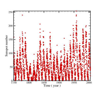
FIG. 1.: Observed spot numbers as a function of time.

In this paper we would like to characterize the complex behavior of sunspot time series through the computation of the signal parameters - scaling exponents - which quantifies the correlation exponents and multifractality of the signal. As shown in Figure 1, the sunspot time series has a sinusoidal trend, with a frequency is equal to the well known cycle of sun activity, approximately $11$years. Because of the nonstationary nature of sunspot time series, and due to the finiteness of the available data sample, we should apply some methods which are insensitive to non-stationarities like trends.

To eliminate the effect of sinusoidal trend, we apply the Fourier Detrended Fluctuation Analysis (F-DFA) [12, 13]. After elimination of the trend we use the Multifractal Detrended Fluctuation Analysis (MF-DFA) to analysis the data set. The MF-DFA methods are the modified version of detrended fluctuation analysis (DFA) to detect multifractal properties of time series. The detrended fluctuation analysis (DFA) method introduced by Peng et al. [14] has became a widely-used technique for the determination of (mono-) fractal scaling properties and the detection of long-range correlations in noisy, nonstationary time series [14, 15, 16, 17, 18]. It has successfully been applied to diverse fields such as DNA sequences [14, 19], heart rate dynamics [20, 21, 22], neuron spiking [23], human gait [24], long-time weather records [25], cloud structure [26], geology [27], ethnology [28], economical time series [29], and solid state physics [30].

The paper is organized as follows: In Section II we describe the MF-DFA and F-DFA methods in detail and show that the scaling exponents determined via the MF-DFA method are identical to those obtained by the standard multifractal formalism based on partition functions. We eliminate the sinusoidal trend via the F-DFA technique in Section III and investigate the multifractal nature of the remaining fluctuation. In Section IV, we examine the source of multifractality in sunspot data by comparison the MF-DFA results for remaining data set to those obtained via the MF-DFA for shuffled and surrogate series. Section V closes with a discussion of the present results.

II Multifractal Detrended Fluctuation Analysis

The simplest type of the multifractal analysis is based upon the standard partition function multifractal formalism, which has been developed for the multifractal characterization of normalized, stationary measurements [31, 32, 33, 34]. Unfortunately, this standard formalism does not give correct results for nonstationary time series that are affected by trends or that cannot be normalized. Thus, in the early 1990s an improved multifractal formalism has been developed, the wavelet transform modulus maxima (WTMM) method [35], which is based on the wavelet analysis and involves tracing the maxima lines in the continuous wavelet transform over all scales. The other method, the multifractal detrended fluctuation analysis (MF-DFA), is based on the identification of scaling of the $q$th-order moments depending on the signal length and is generalization of the standard DFA using only the second moment $q=2$.

The MF-DFA does not require the modulus maxima procedure in contrast WTMM method, and hence does not require more effort in programming and computing than the conventional DFA. On the other hand, often experimental data are affected by non-stationarities like trends, which have to be well distinguished from the intrinsic fluctuations of the system in order to find the correct scaling behavior of the fluctuations. In addition very often we do not know the reasons for underlying trends in collected data and even worse we do not know the scales of the underlying trends, also, usually the available record data is small. For the reliable detection of correlations, it is essential to distinguish trends from the fluctuations intrinsic in the data. Hurst rescaled-range analysis [36] and other non-detrending methods work well if the records are long and do not involve trends. But if trends are present in the data, they might give wrong results. Detrended fluctuation analysis (DFA) is a well-established method for determining the scaling behavior of noisy data in the presence of trends without knowing their origin and shape [14, 21, 37, 38, 39]

A Description of the MF-DFA

The modified multifractal DFA (MF-DFA) procedure consists of five steps. The first three steps are essentially identical to the conventional DFA procedure (see e. g. [14, 15, 16, 17, 18]). Suppose that $x_{k}$ is a series of length $N$, and that this series is of compact support, i.e. $x_{k}=0$ for an insignificant fraction of the values only.

$\bullet$ Step 1: Determine the “profile”

$$Y(i)\equiv\sum_{k=1}^{i}\left[x_{k}-\langle x\rangle\right],\qquad i=1,\ldots,N.$$ (1)

Subtraction of the mean $\langle x\rangle$ is not compulsory, since it would be eliminated by the later detrending in the third step.

$\bullet$ Step 2: Divide the profile $Y(i)$ into $N_{s}\equiv{\rm int}(N/s)$ non-overlapping segments of equal lengths $s$. Since the length $N$ of the series is often not a multiple of the considered time scale $s$, a short part at the end of the profile may remain. In order not to disregard this part of the series, the same procedure is repeated starting from the opposite end. Thereby, $2N_{s}$ segments are obtained altogether.

$\bullet$ Step 3: Calculate the local trend for each of the $2N_{s}$ segments by a least-square fit of the series. Then determine the variance

$$F^{2}(s,\nu)\equiv{1\over s}\sum_{i=1}^{s}\left\{Y[(\nu-1)s+i]-y_{\nu}(i)\right\}^{2},$$ (2)

for each segment $\nu$, $\nu=1,\ldots,N_{s}$ and

$$F^{2}(s,\nu)\equiv{1\over s}\sum_{i=1}^{s}\left\{Y[N-(\nu-N_{s})s+i]-y_{\nu}(i)\right\}^{2},$$ (3)

for $\nu=N_{s}+1,\ldots,2N_{s}$. Here, $y_{\nu}(i)$ is the fitting polynomial in segment $\nu$. Linear, quadratic, cubic, or higher order polynomials can be used in the fitting procedure (conventionally called DFA1, DFA2, DFA3, $\ldots$) [14, 22]. Since the detrending of the time series is done by the subtraction of the polynomial fits from the profile, different order DFA differ in their capability of eliminating trends in the series. In (MF-)DFA$m$ [$m$th order (MF-)DFA] trends of order $m$ in the profile (or, equivalently, of order $m-1$ in the original series) are eliminated. Thus a comparison of the results for different orders of DFA allows one to estimate the type of the polynomial trend in the time series [16, 17].

$\bullet$ Step 4: Average over all segments to obtain the $q$-th order fluctuation function, defined as:

$$F_{q}(s)\equiv\left\{{1\over 2N_{s}}\sum_{\nu=1}^{2N_{s}}\left[F^{2}(s,\nu)\right]^{q/2}\right\}^{1/q},$$ (4)

where, in general, the index variable $q$ can take any real value except zero. For $q=2$, the standard DFA procedure is retrieved. Generally we are interested in how the generalized $q$ dependent fluctuation functions $F_{q}(s)$ depend on the time scale $s$ for different values of $q$. Hence, we must repeat steps 2, 3 and 4 for several time scales $s$. It is apparent that $F_{q}(s)$ will increase with increasing $s$. Of course, $F_{q}(s)$ depends on the DFA order $m$. By construction, $F_{q}(s)$ is only defined for $s\geq m+2$.

$\bullet$ Step 5: Determine the scaling behavior of the fluctuation functions by analyzing log-log plots of $F_{q}(s)$ versus $s$ for each value of $q$. If the series $x_{i}$ are long-range power-law correlated, $F_{q}(s)$ increases, for large values of $s$, as a power-law,

$$F_{q}(s)\sim s^{h(q)}.$$ (5)

In general, the exponent $h(q)$ may depend on $q$. For stationary time series such as fGn (fractional Gaussian noise), $Y(i)$ in Eq. 1, will be a fBm (fractional Brownian motion) signal, so, $0<h(q=2)<1.0$. The exponent $h(2)$ is identical to the well-known Hurst exponent $H$ [14, 15, 31]. Also for a nonstationary signal, such as fBm noise, $Y(i)$ in Eq. 1, will be a sum of fBm signal, so the corresponding scaling exponent of $F_{q}(s)$ is identified by $h(q=2)>1.0$ [14, 40] (see the appendix for more details). In this case the relation between the exponents $h(2)$ and $H$ will be $H=h(q=2)-1$. The exponent $h(q)$ is known as generalized Hurst exponent. The auto-correlation function can be characterized by a power law $C(s)\equiv\langle n_{k}n_{k+s}\rangle\sim s^{-\gamma}$ with exponent $\gamma=2-2H$. Its power spectra can be characterized by $S(\omega)\sim\omega^{-\beta}$ with frequency $\omega$ and $\beta=2H-1$, In the nonstationary case, correlation exponent and power spectrum scaling are $\gamma=-2H$ and $\beta=2H+1$, respectively [14, 40].

For monofractal time series, $h(q)$ is independent of $q$, since the scaling behavior of the variances $F^{2}(s,\nu)$ is identical for all segments $\nu$, and the averaging procedure in Eq. (4) will just give this identical scaling behavior for all values of $q$. If we consider positive values of $q$, the segments $\nu$ with large variance $F^{2}(s,\nu)$ (i. e. large deviations from the corresponding fit) will dominate the average $F_{q}(s)$. Thus, for positive values of $q$, $h(q)$ describes the scaling behavior of the segments with large fluctuations. For negative values of $q$, the segments $\nu$ with small variance $F^{2}(s,\nu)$ will dominate the average $F_{q}(s)$. Hence, for negative values of $q$, $h(q)$ describes the scaling behavior of the segments with small fluctuations [41].

B Relation to standard multifractal analysis

For a stationary, normalized series the multifractal scaling exponents $h(q)$ defined in Eq. (5) are directly related to the scaling exponents $\tau(q)$ defined by the standard partition function-based multifractal formalism as shown below. Suppose that the series $x_{k}$ of length $N$ is a stationary, normalized sequence. Then the detrending procedure in step 3 of the MF-DFA method is not required, since no trend has to be eliminated. Thus, the DFA can be replaced by the standard Fluctuation Analysis (FA), which is identical to the DFA except for a simplified definition of the variance for each segment $\nu$, $\nu=1,\ldots,N_{s}$. Step 3 now becomes [see Eq. (2)]:

$$F_{\rm FA}^{2}(s,\nu)\equiv[Y(\nu s)-Y((\nu-1)s)]^{2}.$$ (6)

Inserting this simplified definition into Eq. (4) and using Eq. (5), we obtain

$$\left\{{1\over 2N_{s}}\sum_{\nu=1}^{2N_{s}}|Y(\nu s)-Y((\nu-1)s)|^{q}\right\}^{1/q}\sim s^{h(q)}.$$ (7)

For simplicity we can assume that the length $N$ of the series is an integer multiple of the scale $s$, obtaining $N_{s}=N/s$ and therefore

$$\sum_{\nu=1}^{N/s}|Y(\nu s)-Y((\nu-1)s)|^{q}\sim s^{qh(q)-1}.$$ (8)

This corresponds to the multifractal formalism used e. g. in [32, 34]. In fact, a hierarchy of exponents $H_{q}$ similar to our $h(q)$ has been introduced based on Eq. (8) in [32]. In order to relate also to the standard textbook box counting formalism [31, 33], we employ the definition of the profile in Eq. (1). It is evident that the term $Y(\nu s)-Y((\nu-1)s)$ in Eq. (8) is identical to the sum of the numbers $x_{k}$ within each segment $\nu$ of size $s$. This sum is known as the box probability $p_{s}(\nu)$ in the standard multifractal formalism for normalized series $x_{k}$,

$$p_{s}(\nu)\equiv\sum_{k=(\nu-1)s+1}^{\nu s}x_{k}=Y(\nu s)-Y((\nu-1)s).$$ (9)

The scaling exponent $\tau(q)$ is usually defined via the partition function $Z_{q}(s)$,

$$Z_{q}(s)\equiv\sum_{\nu=1}^{N/s}|p_{s}(\nu)|^{q}\sim s^{\tau(q)},$$ (10)

where $q$ is a real parameter as in the MF-DFA method, discussed above. Using Eq. (9) we see that Eq. (10) is identical to Eq. (8), and obtain analytically the relation between the two sets of multifractal scaling exponents,

$$\tau(q)=qh(q)-1.$$ (11)

Thus, we observe that $h(q)$ defined in Eq. (5) for the MF-DFA is directly related to the classical multifractal scaling exponents $\tau(q)$. Note that $h(q)$ is different from the generalized multifractal dimensions

$$D(q)\equiv{\tau(q)\over q-1}={qh(q)-1\over q-1},$$ (12)

that are used instead of $\tau(q)$ in some papers. While $h(q)$ is independent of $q$ for a monofractal time series, $D(q)$ depends on $q$ in this case. Another way to characterize a multifractal series is the singularity spectrum $f(\alpha)$, that is related to $\tau(q)$ via a Legendre transform [31, 33],

$$\alpha=\tau^{\prime}(q)\quad{\rm and}\quad f(\alpha)=q\alpha-\tau(q).$$ (13)

Here, $\alpha$ is the singularity strength or Hölder exponent, while $f(\alpha)$ denotes the dimension of the subset of the series that is characterized by $\alpha$. Using Eq. (11), we can directly relate $\alpha$ and $f(\alpha)$ to $h(q)$,

$$\alpha=h(q)+qh^{\prime}(q)\quad{\rm and}\quad f(\alpha)=q[\alpha-h(q)]+1.$$ (14)

A Hölder exponent denotes monofractality, while in the multifractal case, the different parts of the structure are characterized by different values of $\alpha$, leading to the existence of the spectrum $f(\alpha)$.

C Fourier-Detrended Fluctuation Analysis

In some cases, there exist one or more crossover (time) scales $s_{\times}$ separating regimes with different scaling exponents [16, 17]. In this case investigation of the scaling behavior is more complicate and different scaling exponents are required for different parts of the series [18]. Therefore one needs a multitude of scaling exponents (multifractality) for a full description of the scaling behavior. A crossover usually can arise from a change in the correlation properties of the signal at different time or space scales, or can often arise from trends in the data. To remove the crossover due to a trend such as sinusoidal trends, Fourier-Detrende Fluctuation Analysis (F-DFA) is applied. The F-DFA is a modified approach for the analysis of low frequency trends added to a noise in time series [12, 13, 42, 43].

In order to investigate how we can remove trends having a low frequency periodic behavior, we transform data record to Fourier space, then we truncate the first few coefficient of the Fourier expansion and inverse Fourier transform the series. After removing the sinusoidal trends we can obtain the fluctuation exponent by using the direct calculation of the MF-DFA. If truncation numbers are sufficient, The crossover due to a sinusoidal trend in the log-log plot of $F_{q}(s)$ versus $s$ disappears.

III Analysis of sunspot time series

As mentioned in section II, a spurious of correlations may be detected if time series is nonstationarity, so direct calculation of correlation behavior, spectral density exponent, fractal dimensions etc., don’t give the reliable results. It can be checked that the sunspot time series is nonstationary. One can verified the non-stationarity property experimentally by measuring the stability of the average and variance in a moving window for example with scale $s$. Figure 2 shows the standard deviation of signal verses scale $s$ isn’t saturate. Let us determine that whether the data set has a sinusoidal trend or not. According to the MF-DFA1 method, Generalized Hurst exponents $h(q)$ in Eq. (5) can be found by analyzing log-log plots of $F_{q}(s)$ versus $s$ for each $q$. Our investigation shows that there are three crossover time scales $s_{\times}$ in the log-log plots of $F_{q}(s)$ versus $s$ for every $q$’s. These three crossovers divide $F_{q}(s)$ into four regions, as shown in Figure 3 ( for instance we took $q=2$). The existence of these regions is due to the competition between noise and sinusoidal trend. For $s<s_{1\times}$ and $s>s_{3\times}$, the noise has the dominating effect [17]. For $s_{1\times}<s<s_{2\times}$ and $s_{2\times}<s<s_{3\times}$, the sinusoidal trend dominates [17]. The value of $s_{2\times}$ is approximately equal to $130$ month which is equal to the well known cycle of sun activity. As mentioned before, for very small scales $s<s_{1\times}$ the effect of the sinusoidal trend is not pronounced, indicating that in this scale region the signal can be considered as noise fluctuating around a constant which is filtered out by the MF-DFA1 procedure. In this region the generalized DFA1 exponent is $h(q=2)=1.12\pm 0.01$, where confirms that the process is a non-stationary process with anti-correlation behavior.

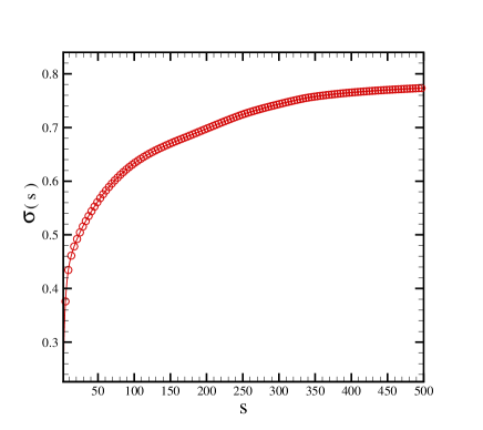
FIG. 2.: Behavior of standard deviation of sunspot time series as a function of time scale. It shows that this time series is not stationary and direct calculation of correlation gives strongly wrong result.

To cancel the sinusoidal trend in MF-DFA1, we apply F-DFA method for sunspot data. We truncate some of the first coefficient of the Fourier expansion of sunspot series. According to Figure 4, for eliminating the crossover scales, we need to remove approximately $50$ terms of the Fourier expansion. Then, by inverse Fourier Transformation, the noise without sinusoidal trend is extracted.

The MF-DFA1 results of the remanning new signal are shown in Figure 5. The sunspot time series is a multifractal process as indicated by the strong $q$ dependence of generalized Hurst exponents and $\tau(q)$[44]. The $q$- dependence of the classical multifractal scaling exponent $\tau(q)$ has different behaviors for $q<0$ and $q>0$. For positive and negative values of $q$, the slopes of $\tau(q)$ are $1.11\pm 0.01$ and $1.44\pm 0.01$, respectively. According to the relation between the Hurst exponent and $h(2)$, i.e. $h(q=2)-1=H$, we find that the Hurst exponent is $0.12\pm 0.01$. This result is equal to value of Hurst exponent in small scale of MF-DFA1 of noise with sinusoidal trend. The fractal dimension is obtained as $D_{f}=2-H=1.88$ [16]. The values of derived quantities from MF-DFA1 method, are given in Table II and Table III.

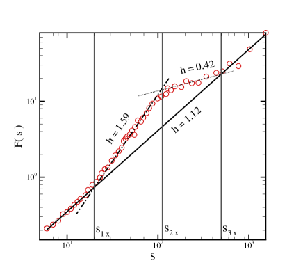
FIG. 3.: Crossover behavior of log-log plot $F(s)$ versus $s$ for sunspot time series for $q=2.0$. There are three crossover time scales in plot of $F(s)$, at scales $s_{1\times}$, $s_{2\times}$ and $s_{3\times}$.

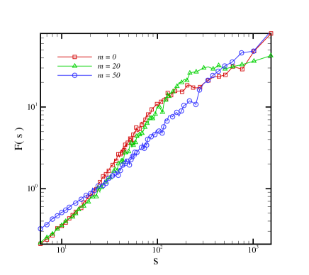
FIG. 4.: The MF-DFA1 functions $F_{q}(s)$ for sunspot time series versus the time scale $s$ in log-log plot. Original time series $m=0$, truncation of the first $20$ terms $m=20$ and $50$ terms $m=50$.

Usually, in the MF-DFA method, deviation from a straight line in the log-log plot of Eq. (5) occurs for small scales $s$. This deviation limits the capability of DFA to determine the correct correlation behavior for very short scales and in the regime of small $s$. The modified MF-DFA is defined as follows [16]:

$$F^{\rm mod}_{q}(s) = \frac{F_{q}(s)}{K_{q}(s)},$$ (15)

$$= F_{q}(s){\langle[F_{q}^{\rm shuf}(s^{\prime})]^{2}\rangle^{1/2}\,s^{1/2}\over\langle[F_{q}^{\rm shuf}(s)]^{2}\rangle^{1/2}\,s^{\prime 1/2}}\quad{\rm(for}\,s^{\prime}\gg 1),$$ (16)

where $\langle[F_{q}^{\rm shuf}(s)]^{2}\rangle^{1/2}$ denotes the usual MF-DFA fluctuation function [defined in Eq. (4)] averaged over several configurations of shuffled data taken from the original time series, and $s^{\prime}\approx N/40$. The values of the Hurst exponent obtained by modified MF-DFA1 methods for sunspot time series is $0.11\pm 0.01$. The relative deviation of the Hurst exponent which is obtained by modified MF-DFA1 in comparison to MF-DFA1 for original data is approximately $8.33\%$.

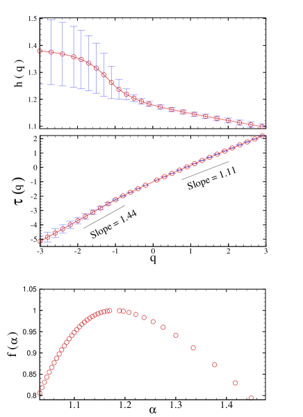
FIG. 5.: The $q$ dependence of the generalized Hurst exponent $h(q)$, the corresponding $\tau(q)$ and singularity spectrum $f(\alpha)$ are shown in the upper to lower panel respectively for sunspot time series without sinusoidal trend.

TABLE I.: The values of the Hurst, multifractal scaling and generalized multifractal exponents for $q=2.0$, for original, surrogate and shuffled of temperature fluctuation series obtained by MF-DFA1.

Data	$H$	$\tau$	$D$
CMB	$0.94\pm 0.01$	$0.88\pm 0.02$	$0.88\pm 0.02$
Surrogate	$0.88\pm 0.01$	$0.76\pm 0.02$	$0.76\pm 0.02$
Shuffled	$0.50\pm 0.001$	$0.002\pm 0.002$	$0.002\pm 0.002$

IV Comparison of the multifractality for original, shuffled and surrogate sunspot time series

As discussed in the section III the remanning data set after the elimination of sinusoidal trend has the multifractal nature. In this section we are interested in to determine the source of multifractality. In general, two different types of multifractality in time series can be distinguished: (i) Multifractality due to a fatness of probability density function (PDF) of the time series. In this case the multifractality cannot be removed by shuffling the series. (ii) Multifractality due to different correlations in small and large scale fluctuations. In this case the data may have a PDF with finite moments, e. g. a Gaussian distribution. Thus the corresponding shuffled time series will exhibit mono-fractal scaling, since all long-range correlations are destroyed by the shuffling procedure. If both kinds of multifractality are present, the shuffled series will show weaker multifractality than the original series. The easiest way to clarify the type of multifractality, is by analyzing the corresponding shuffled and surrogate time series. The shuffling of time series destroys the long range correlation, Therefore if the multifractality only belongs to the long range correlation, we should find $h_{\rm shuf}(q)=0.5$. The multifractality nature due to the fatness of the PDF signals is not affected by the shuffling procedure. On the other hand, to determine the multifractality due to the broadness of PDF, the phase of discrete fourier transform (DFT) coefficients of sunspot time series are replaced with a set of pseudo independent distributed uniform $(-\pi,\pi)$ quantities in the surrogate method. The correlations in the surrogate series do not change, but the probability function changes to the Gaussian distribution. If multifractality in the time series is due to a broad PDF, $h(q)$ obtained by the surrogate method will be independent of $q$. If both kinds of multifractality are present in sunspot time series, the shuffled and surrogate series will show weaker multifractality than the original one.

To check the nature of multifractality, we compare the fluctuation function $F_{q}(s)$, for the original series ( after cancelation of sinusoidal trend) with the result of the corresponding shuffled, $F_{q}^{\rm shuf}(s)$ and surrogate series $F_{q}^{\rm sur}(s)$. Differences between these two fluctuation functions with the original one, directly indicate the presence of long range correlations or broadness of probability density function in the original series. These differences can be observed in a plot of the ratio $F_{q}(s)/F_{q}^{\rm shuf}(s)$ and $F_{q}(s)/F_{q}^{\rm sur}(s)$ versus $s$ [44]. Since the anomalous scaling due to a broad probability density affects $F_{q}(s)$ and $F_{q}^{\rm shuf}(s)$ in the same way, only multifractality due to correlations will be observed in $F_{q}(s)/F_{q}^{\rm shuf}(s)$. The scaling behavior of these ratios are

$$F_{q}(s)/F_{q}^{\rm shuf}(s)\sim s^{h(q)-h_{\rm shuf}(q)}=s^{h_{\rm cor}(q)},$$ (18)

$$F_{q}(s)/F_{q}^{\rm sur}(s)\sim s^{h(q)-h_{\rm sur}(q)}=s^{h_{\rm PDF}(q)}.$$ (19)

If only fatness of the PDF is responsible for the multifractality, one should find $h(q)=h_{\rm shuf}(q)$ and $h_{\rm cor}(q)=0$. On the other hand, deviations from $h_{\rm cor}(q)=0$ indicates the presence of correlations, and $q$ dependence of $h_{\rm cor}(q)$ indicates that multifractality is due to the long rage correlation. If only correlation multifractality is present, one finds $h_{\rm shuf}(q)=0.5$. If both distribution and correlation multifractality are present, both, $h_{\rm shuf}(q)$ and $h_{\rm sur}(q)$ will depend on $q$. The $q$ dependence of the exponent $h(q)$ for original, surrogate and shuffled time series are shown in Figures 6. The $q$ dependence of $h_{\rm cor}$ and $h_{\rm PDF}$ shows that the multifractality nature of sunspot time series is due to both broadness of the PDF and long range correlation. The absolute value of $h_{\rm cor}(q)$ is greater than $h_{\rm PDF}(q)$, so the multifractality due to the fatness is weaker than the mulifractality due to the correlation. The deviation of $h_{\rm sur}(q)$ and $h_{\rm shuf}(q)$ from $h(q)$ can be determined by using $\chi^{2}$ test as follows:

$$\chi^{2}_{\diamond}=\sum_{i=1}^{N}\frac{[h(q_{i})-h_{\diamond}(q_{i})]^{2}}{\sigma(q_{i})^{2}+\sigma_{\diamond}(q_{i})^{2}},$$ (20)

the symbol $"\diamond"$ can be replaced by $"\rm sur"$ and $"\rm shuf"$, to determine the confidence level of $h_{\rm sur}$ and $h_{\rm shuf}$ to generalized Hurst exponents of original series, respectively. The value of reduced chi-square $\chi^{2}_{\nu\diamond}=\frac{\chi^{2}_{\diamond}}{\cal{N}}$ ($\cal{N}$ is the number of degree of freedom) for shuffled and surrogate time series are $1653.47$, $1.10$, respectively. On the other hand the width of singularity spectrum, $f(\alpha)$, i.e. $\Delta\alpha=\alpha(q_{min})-\alpha(q_{max})$ for original, surrogate and shuffled time series are approximately, $0.44$, $0.75$ and $0.22$ respectively. These values also show that the multifractality due to correlation is dominant[45].

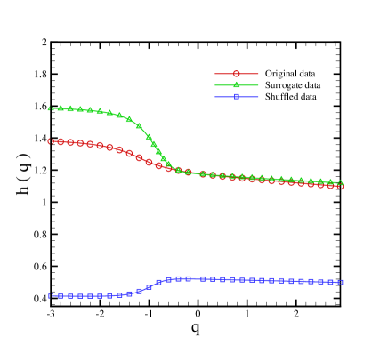
FIG. 6.: Generalized Hurst exponent, $h(q)$ as a function of $q$ for original, surrogate and shuffled data.

The values of the generalized Hurst exponent $h(q=2.0)$, multifractal scaling $\tau(q=2)$ and generalized multifractal exponents $(D(q=2))$ for the original, shuffled and surrogate of sunspot time series obtained with MF-DFA1 method are reported in Table II, The related scaling exponents are indicated in Table III. The values of the Hurst exponent obtained by MF-DFA1 and modified MF-DFA1 methods for original, surrogate and shuffled sunspot time series are given in Table IV.

V Conclusion

The MF-DFA method allows us to determine the multifractal characterization of the nonstationary and stationary time series. The concept of MF-DFA of sunspot time series can be used to gain deeper insight in to the processes occurring in nonstationary dynamical system such as sunspots formation. We have shown that the MF-DFA1 result of the monthly sunspot time series has three crossover time scale $(s_{\times})$. These crossover time scale are due to the sinusoidal trend. To minimizing the effect of this trend, we have applied F-DFA on sunspot time series. Applying the MF-DFA1 method on truncated data, demonstrated that the monthly sunspot time series is a nonstationary time series with anti-correlation behavior. The $q$ dependence of $h(q)$ and $\tau(q)$, indicated that the monthly sunspot time series has multifractal behavior. By comparing the generalized Hurst exponent of the original time series with the shuffled and surrogate one’s, we have found that multifractality due to the correlation has more contribution than the broadness of the probability density function.

TABLE II.: The values of $h(q=2)$, multifractal scaling and generalized multifractal exponents for $q=2.0$ for original, surrogate and shuffled of monthly sunspot time series obtained by MF-DFA1.

Data	$h$	$\tau$	$D$
Sunspot	$1.12\pm 0.01$	$1.24\pm 0.02$	$1.24\pm 0.02$
Surrogate	$1.13\pm 0.01$	$1.26\pm 0.02$	$1.26\pm 0.02$
Shuffled	$0.51\pm 0.01$	$0.02\pm 0.02$	$0.02\pm 0.02$

TABLE III.: The values of the Hurst $(H)$, power spectrum scaling $(\beta)$ and auto-correlation scaling $(\gamma)$ exponents for original, surrogate and shuffled of monthly sunspot time series obtained by MF-DFA1.

Data	$H$	$\beta$	$\gamma$
Sunspot	$0.12\pm 0.02$	$1.24\pm 0.02$	$-0.24\pm 0.02$
Surrogate	$0.13\pm 0.02$	$1.26\pm 0.02$	$-0.26\pm 0.02$
Shuffled	$0.51\pm 0.01$	$0.02\pm 0.02$	$0.98\pm 0.02$

TABLE IV.: The value of the Hurst exponent using MF-DFA1 and modified MF-DFA1 for the original, shuffled and surrogate of monthly sunspot time series.

Method	Sunspot	Surrogate	Shuffled
MF-DFA1	$0.12\pm 0.01$	$0.13\pm 0.01$	$0.51\pm 0.01$
Modified	$0.11\pm 0.01$	$0.12\pm 0.01$	$0.50\pm 0.01$

Acknowledgements We would like to thank Sepehr Arbabi Bidgoli and Mojtaba Mohammadi Najafabadi for reading the manuscript and useful comments. This paper is dedicated to Dr. Somaihe Abdolahi.

VI APPENDIX

In this appendix we derive the relation between the exponent $h(2)$ (DFA1 exponent) and Hurst exponent of a fBm signal. We show that for such nonstationary signal the average sample variance (Eq. 4) for $q=2$, is proportional to $s^{h(q)}$, where $h(q=2)=H+1$. It is shown that the averaged sample variance $F^{2}(s)$ behaves as:

$$F^{2}(s) \equiv \frac{1}{2N_{s}}\sum_{\nu=1}^{2N_{s}}\left[F^{2}(s,\nu)\right],$$ (21)

$$= \left\langle\left[F^{2}(s,\nu)\right]\right\rangle_{\nu},$$ (22)

$$\equiv {\mathcal{C}_{H}}s^{2(H+1)},$$ (23)

where $F^{2}(s,\nu)$ is defined as Eq. 2 and ${\mathcal{C}_{H}}$ is a function of Hurst exponent $H$.

To prove the statement we note that the data $x(k)$ is a fractional Brownian motion (fBm), the partial sums $Y(i)$ (Eq. 1) will be a summed fBm signal. In the DFA1, the fitting function will have the expression $(y_{\nu}=a_{\nu}+b_{\nu}i)$. The slope $b_{\nu}$ and intercept $a_{\nu}$ of a least-squares line on $Y(i)$ (from $0$ to $s$) for every windows $(\nu)$ are given by

$$b_{\nu} = \frac{\sum_{i=1}^{s}Y(i)i-\frac{1}{s}\sum_{i=1}^{s}Y(i)\sum_{i=1}^{s}i}{\sum_{i=1}^{s}i^{2}-\frac{1}{s}\left[\sum_{i=1}^{s}i\right]^{2}},$$ (25)

$$\simeq\frac{\sum_{i=1}^{s}Y(i)i-\frac{s}{2}\sum_{i=1}^{s}Y(i)}{s^{3}/12}$$

$$a_{\nu} = \frac{1}{s}\sum_{i=1}^{s}Y(i)-\frac{1}{s}\sum_{i=1}^{s}i\simeq\frac{1}{s}\sum_{i=1}^{s}Y(i)-\frac{s}{2},$$ (26)

respectively.

Using the Eqs. 4 and 26, the Eq. 23 can be written as follows

$$\left\langle\left[F^{2}(s,\nu)\right]\right\rangle=\left\langle\frac{1}{s}\sum_{i=1}^{s}(Y(i)-a-bi)^{2}\right\rangle$$ (27)

$$\simeq \left\langle\frac{1}{s}\sum_{i=1}^{s}Y(i)^{2}\right\rangle+\left\langle a^{2}\right\rangle+\frac{s^{2}}{3}\left\langle b^{2}\right\rangle$$ (29)

$$-2\left\langle\frac{a}{s}\sum_{i=1}^{s}y(i)\right\rangle-2\left\langle\frac{b}{s}\sum_{i=1}^{s}iY(i)\right\rangle+s\left\langle ab\right\rangle,$$

$$= \left\langle\frac{1}{s}\sum_{i=1}^{s}Y(i)^{2}\right\rangle-\frac{4}{s^{2}}\left\langle\left[\sum_{i=1}^{s}Y(i)\right]^{2}\right\rangle$$ (31)

$$-\frac{12}{s^{4}}\left\langle\left[\sum_{i=1}^{s}iY(i)\right]^{2}\right\rangle+\frac{12}{s^{3}}\left\langle\sum_{i=1}^{s}iY(i)\sum_{i=1}^{s}Y(i)\right\rangle,$$

$$= \frac{A}{s}-\frac{4}{s^{2}}B-\frac{12}{s^{4}}D+\frac{12}{s^{3}}C.$$ (32)

where we have discard the subscript $\nu$ for simplicity. Now let us calculate the functions $A$, $B$, $C$ and $D$ in Eq. 32. The increment of a summed fBm and fBm signals, i.e.

$$x(i)=Y(i)-Y(i-1)$$ (33)

$$u(i)=x(i)-x(i-1)$$ (34)

are a fBm $x(i)$ and fGn $u(i)$ noise, respectively. The correlation of $Y(i)$ and $x(i)$ are as follows [15]

$$\left\langle x(i)x(j)\right\rangle = \frac{\sigma^{2}}{2}\left[i^{2H}+j^{2H}-|i-j|^{2H}\right],$$ (35)

$$\left\langle Y(i)Y(j)\right\rangle = \frac{\sigma^{2}}{(H+1)^{2}}\left(ij\right)^{H+1},$$ (36)

where $\sigma^{2}=\left\langle u(i)^{2}\right\rangle$. Also the variance of a summed fBm signal is $\left\langle Y(i)^{2}\right\rangle=\frac{\sigma^{2}}{(H+1)^{2}}i^{2(H+1)}$ [14]. Finlly using the Eqs. 26 and 36, it can be easily shown that the Eq. 32 can be written as follows

$$\left\langle\left[F^{2}(s,\nu)\right]\right\rangle_{\nu}={\mathcal{C}_{H}}s^{2(H+1)},$$ (37)

where ${\mathcal{C}_{H}}$ is

$${\mathcal{C}_{H}} = \frac{\sigma^{2}}{(2H+3)(H+1)^{2}}-\frac{4\sigma^{2}}{[(H+1)(H+2)]^{2}}$$ (39)

$$-\frac{12\sigma^{2}}{[(H+1)(H+3)]^{2}}+\frac{12\sigma^{2}}{(H+1)^{2}(H+2)(H+3)}.$$

Therefore the standard DFA$1$ exponent for a nonstationary signal is related to its Hurst exponent as $h(q=2)=H+1$.

REFERENCES

- [1] Bray R J and Loughhead R E, 1979 Sunspots(Dover Publications, New York).
- [2] Petrovaye E, 2000 ESA Publ. Solar Physics, 463, 3-14
- [3] http://www.oma.be/KSB-ORB/SIDC/index.html
- [4] Veronig A, Messerotti M and Hanslmeier A, 2000 Astronomy and Astrophysics, 357, 337-350
- [5] Abramenko V I, 2005 Solar Physics, 228, 29-42
- [6] Zhukov V I, [arXive:astro-ph/0304456].
- [7] Temmer M, Veronig A, Rybák J and Hanslmeier A, Solar variability: from core to outer frontiers, 2002 10th Eur. Solar Physics Mtg (9 14 September 2002, Prague, Czech Republic) vol 2, ESA SP-506, ed A Wilson (Noordwijk: ESA Publications Division) pp 859 62
- [8] Temmer M, Veronig A and Hanslmeier A, 2002 Astronomy and Astrophysics, 390, 707-715
- [9] Bogart R S, 1982 Solar Physics, 76, 155
- [10] Temmer M and et. al., [arXive:astro-ph/0207239].
- [11] Temmer M, Veronig A and Hanslmeier A, 2003 Solar Physics, 512, 111-129
- [12] Nagarajan R and Kavasseri R G, [arXive:cond-mat/0411543]
- [13] Chianca C V, Ticona A and Penna T J P, 2005 Physica A, 357, 447-454
- [14] Peng C K, Buldyrev S V, Havlin S, Simons M, Stanley H E, and Goldberger A L, 1994 Phys. Rev. E 49, 1685 ; Ossadnik S M, Buldyrev S B, Goldberger A L, Havlin S, Mantegna R N, Peng C K, Simons M and Stanley H E, 1994 Biophys. J. 67, 64
- [15] Taqqu M S, Teverovsky V and Willinger W, 1995 Fractals 3, 785
- [16] Kantelhardt J W, Koscielny-Bunde E, Rego H H A, Havlin S and Bunde A, 2001 Physica A 295, 441
- [17] Hu K, Ivanov P Ch, Chen Z, Carpena P and Stanley H E, 2001 Phys. Rev. E 64, 011114
- [18] Chen Z, Ivanov P Ch, Hu K and Stanley H E, 2002 Phys. Rev. E 65, preprint physics/0111103.
- [19] Buldyrev S V, Goldberger A L, Havlin S, Mantegna R N, Matsa M E, Peng C K, Simons M and Stanley H E, 1995 Phys. Rev. E 51, 5084; Buldyrev S V, Dokholyan N V, Goldberger A L, Havlin S, Peng C K, Stanley H E and Viswanathan G M, 1998 Physica A 249, 430
- [20] Ivanov P Ch, Bunde A, Amaral L A N, Havlin S, Fritsch-Yelle J, Baevsky R M, Stanley H E and Goldberger A L, 1999 Europhys. Lett. 48, 594; Ashkenazy Y, Lewkowicz M, Levitan J, Havlin S, Saermark K, Moelgaard H, Thomsen P E B, Moller M, Hintze U and Huikuri H V, 2001 Europhys. Lett. 53, 709; Ashkenazy Y, Ivanov P Ch, Havlin S, Peng C K, Goldberger A L and Stanley H E, 2001 Phys. Rev. Lett. 86, 1900
- [21] Peng C K, Havlin S, Stanley H E and Goldberger A L, 1995 Chaos 5 82
- [22] Bunde A, Havlin S, Kantelhardt J W, Penzel T, Peter J H and Voigt K, 2000 Phys. Rev. Lett. 85, 3736
- [23] Blesic S, Milosevic S, Stratimirovic D and Ljubisavljevic M, 1999 Physica A 268, 275; Bahar S, Kantelhardt J W, Neiman A, Rego H H A, Russell D F, Wilkens L, Bunde A and Moss F, 2001 Europhys. Lett. 56, 454
- [24] Hausdorff J M, Mitchell S L, Firtion R, Peng C K, Cudkowicz M E, Wei J Y and Goldberger A L, 1997 J. Appl. Physiology 82, 262
- [25] Koscielny-Bunde E, Bunde A, Havlin S, Roman H E, Goldreich Y and Schellnhuber H J, 1998 Phys. Rev. Lett. 81, 729; Ivanova K and Ausloos M, 1999 Physica A 274, 349; Talkner P and Weber R O, 2000 Phys. Rev. E 62, 150
- [26] Ivanova K, Ausloos M, Clothiaux E E and Ackerman T P, 2000 Europhys. Lett. 52, 40
- [27] Malamud B D and Turcotte D L, 1999 J. Stat. Plan. Infer. 80, 173
- [28] Alados C L and Huffman M A, 2000 Ethnology 106, 105
- [29] Mantegna R N and Stanley H E, 2000 An Introduction to Econophysics (Cambridge University Press, Cambridge); Liu Y, Gopikrishnan P, Cizeau P, Meyer M, Peng C K and Stanley H E, 1999 Phys. Rev. E 60, 1390; Vandewalle N, Ausloos M and Boveroux P, 1999 Physica A 269, 170
- [30] Kantelhardt J W, Berkovits R, Havlin S and Bunde A, 1999 Physica A 266, 461; Vandewalle N, Ausloos M, Houssa M, Mertens P W and Heyns M M, 1999 Appl. Phys. Lett. 74, 1579
- [31] Feder J, 1988 Fractals (Plenum Press, New York)
- [32] Barabási A L and Vicsek T, 1991 Phys. Rev. A 44, 2730
- [33] Peitgen H O, Jürgens H and Saupe D, 1992 Chaos and Fractals (Springer-Verlag, New York), Appendix B
- [34] Bacry E, Delour J and Muzy J F, 2001 Phys. Rev. E 64, 026103
- [35] Muzy J F, Bacry E and Arneodo A, 1991 Phys. Rev. Lett. 67, 3515
- [36] Hurst H E, Black R P and Simaika Y M, 1965 Long-term storage. An experimental study (Constable, London)
- [37] Fano U, 1947 Phys. Rev. 72 26
- [38] Barmes J A and Allan D W, 1996 Proc. IEEE 54 176
- [39] Buldyrev S V, Goldberger A L, Havlin S, Mantegna R N, Matsa M E, Peng C K, Simons M, Stanley H E, 1995 Phys. Rev. E 51 5084
- [40] Eke A, Herman P, Kocsis L and Kozak L R, 2002 Physiol. Meas. 23, R1-R38
- [41] For the maximum scale the fluctuation function is independent of , since the sum in Eq. (4) runs over only two identical segments (). For smaller scales the averaging procedure runs over several segments, and the average value will be dominated by the from the segments with small (large) fluctuations if (). Thus, for , with will be smaller than with , while both become equal for . Hence, if we assume an homogeneous scaling behavior of following Eq. (5), the slope in a log-log plot of with versus must be larger than the corresponding slope for with . Thus, for will usually be larger than for .
- [42] Koscielny-Bunde E, Roman H E, Bunde A, Havlin S and Schellnhuber H J, 1998 Phil. Mag. B 77 1331
- [43] Koscielny-Bunde E, Bunde A, Havlin S, Roman H E, Goldreich Y and Schellnhuber H J, 1998 Phys. Rev. Lett. 81 729.
- [44] Gantelhardt J W, Zschiegner S A, Kosciliny-Bunde E, Bunde A, Pavlin S and Stanley H E, 2002 Physica A 316, 78-114
- [45] Oświȩcimka P and et. al, [arXive:cond-mat/0504608]