Siegert pseudostate perturbation theory: one- and two-threshold cases

Abstract

Perturbation theory for the Siegert pseudostates (SPS) [Phys. Rev. A58, 2077 (1998) and Phys. Rev. A67, 032714 (2003)] is studied for the case of two energetically separated thresholds. The perturbation formulas for the one-threshold case are derived as a limiting case whereby we reconstruct More’s theory for the decaying states [Phys. Rev. A3, 1217 (1971)] and amend an error. The perturbation formulas for the two-threshold case have additional terms due to the non-standard orthogonality relationship of the Siegert Pseudostates. We apply the theory to a 2-channel model problem, and find the rate of convergence of the perturbation expansion should be examined with the aide of the variance $D=||E-\sum_{n}\lambda^{n}E^{(n)}||$ instead of the real and imaginary parts of the perturbation energy individually.

I INTRODUCTION

Resonances occur in a variety of fields of physical sciences. Despite their diversity, they are characterized by two parameters, the resonance energy position and width, apart from the coupling with the background continuum represented by the Fano profilefano-rau . A great deal of discussions have been given to the interpretation of resonance phenomenafano-rau . The most familiar parameterization of the resonances is condensed into the dispersion formula due to Breit and Wigner. Back in 1939, Siegert Siegert developed a compact mathematical viewpoint for characterizing resonances as singular points of the dispersion relation. His idea requires the solution of the Schrödinger equation subject to the outgoing wave boundary condition,

$$\left.\left(\frac{d}{dr}-ik\right)\phi(r)\right|_{r=a}=0,$$

where $a$ is the radius beyond which the potential energy is negligible. The solution $\phi(r)$ is called the Siegert state (SS) and it behaves like ${\rm e}^{ikr}$ near $r=a$ and beyond. This boundary condition destroys the hermiticity of the Hamiltonian, thus entailing complex-valued eigenenergies, i.e.,

$$E=\frac{k^{2}}{2}=E_{\rm res}-i\frac{\Gamma}{2}$$

This is a most direct representation of both the resonance position and width. This mathematically appealing representation had been implemented with tedious iterations due to lack of suitable computational techniques until Tolstikhin et al oleg made a breakthrough by introducing Siegert pseudostates (SPS) for the one-threshold case. Their idea incorporates the boundary condition into the Schrödinger equation so that the dispersion relation is obtained by a single diagonalization of the Hamiltonian matrix. Previous applications of SPS to resonances in three-body Coulomb problems indicate that it is not only a valid procedure but also a new perspective for the SPS representation of resonances and decay processes olegclmb . Another immediate application of the SPS theory is to the time-dependent problemtime-dept ; CHG where the reflection off the exterior boundary incurs numerical instability. Tanabe and Watanabe tana-wata succeeded in describing the reflectionless time propagation based on the Siegert pseudostates. Indeed, applied to the half-cycle optical pulses, the Siegert boundary condition indeed was seen to eliminate the outgoing wave component perfectly.

Recently, Sitnikov and Tolstikhin sit-tol ; toyota stretched the scope of the SPS theory by enabling the treatment of the two-threshold problem. Despite such progress, there remains in the theory of SPS a chapter still incompletely worked out. This is the Siegert perturbation theory. A pioneering work on this subject is due to Moremore1 ; more2 who extended the Siegert state theory specifically to handle the decaying state. The main purpose of this paper is to complete the Siegert perturbation theory from the recently developed SPS viewpoint for both one- and two-threshold cases. Particularly, in the one-threshold case, we are able to reconstruct More’s theory for decaying states more1 in terms of SPS but with an unexpected amendment to his theory. The SPS perturbation theory (SPSPT) is by no means straightforward owing to the non-standard orthonormality of the eigenfunctions. This constraint also serves to fix the phase of the perturbed wavefunction, a feature which is absent from the standard perturbation theory. It is hoped this paper serves to expose such noteworthy features of the SPSPT.

This paper is thus constructed as follows. In Section II, we review some basic ideas about the SPS as needed for an elementary presentation of the perturbation theory. Section III gives the details of the SPSPT for both one- and two-threshold cases. And Section III deals with a specific mathematical model as an example of the SPSPT. Atomic units are used throughout.

II THE SIEGERT PSEUDOSTATES

Since the two-threshold SPS theory contains the one-threshold case in itself, we review the two-threshold case only, leaving the one-threshold case as the limit where the two-thresholds become degenerate sit-tol .

II.1 Mathematical Settings

Suppose first that there are as many as $q$ independent channels. The Schrödinger equation reads

$$\left[-\frac{1}{2}\frac{d^{2}}{dr^{2}}+V(r)-E\right]\phi(r)=0,$$ (1)

where

$$V(r) = \left(\begin{array}[]{cccc}V_{1}&V_{12}&\cdots&V_{1q}\\ V_{12}&V_{2}&\cdots&V_{2q}\\ \vdots&\vdots&\ddots&\vdots\\ V_{1q}&V_{2q}&\cdots&V_{q}\\ \end{array}\right),$$

$$\phi(r) = \left(\begin{array}[]{c}\phi_{1}\\ \phi_{2}\\ \vdots\\ \phi_{q}\end{array}\right)$$

and $V_{i}$ pertains to the potential energy of channel $i$, and $V_{ij}$ represents the interchannel coupling between channels $i$ and $j$. We consider the situation where there are only two energetically distinct thresholds so that we separate $V_{i}$ into two groups. A first group contains channels $1,\ldots,q_{1}$ and they converge to $v_{1}$ as $r\to a$ while the other group contains channels $q_{1}+1,\ldots,q$ and they converge to $v_{2}$, that is

$$\lim_{r\rightarrow a}V(r)={\rm diag}[\overbrace{v_{1},\cdots,v_{1}}^{1,\cdots,q_{1}},\overbrace{v_{2},\cdots,v_{2}}^{q_{1}+1,\ldots,q}],$$

where $v_{1}$ and $v_{2}$ are the two constants representing the threshold energies. This allows us to use the 2-channel SPS scheme even in the presence of more than two channels. The two channel momenta are $k_{1}=\sqrt{2(E-v_{1})}$ and $k_{2}=\sqrt{2(E-v_{2})}$. The boundary conditions are thus

$$\phi_{i}(0)=0$$

at $r=0$ and

$$\left.\left(\frac{d}{dr}-ik_{j}\right)\phi_{i}\right|_{r=a}=0$$

at $r=a$ where $j=1$ for the first group, $i=1,\ldots,q_{1}$, and $j=2$ for the second group, $i=q_{1}+1,\ldots,q$. Now, consider to expand the wavefunction $\phi_{i}$ by a complete orthonormal basis set $\{\pi_{l}(r),(l=1,...,N)\}$ over $r\in[0,a]$ such that

$$\phi_{i}(r)=\sum_{l=1}^{N}c_{i,l}\pi_{l}(r).$$

Substituting this into Eq. (1), and integrating over the interval $[0,a]$, we obtain the $M=q\times N$-dimensional eigen value problem,

$$\left[\tilde{H}-\frac{i}{2}B-EI_{M}\right]\vec{c}=0,$$ (4)

where

$$\tilde{H} = \left(\begin{array}[]{cccc}\tilde{H}^{(1)}&U^{(12)}&\cdots&U^{(1q)}\\ U^{(12)}&\tilde{H}^{(2)}&\cdots&U^{(2q)}\\ \vdots&\vdots&\ddots&\vdots\\ U^{(q1)}&U^{(q2)}&\cdots&\tilde{H}^{(q)}\end{array}\right),$$

$$B=\bordermatrix{&1&\cdots&q_{1}&q_{1}+1&\cdots&q{\rm-th\ block}\cr&k_{1}L\cr&&\ddots&&&0\cr&&&k_{1}L&&\cr&&&&k_{2}L&\cr&&0&&&\ddots\cr&&&&&&k_{2}L}$$

$$\vec{c} = \left(\begin{array}[]{c}c_{1,1}\\ \vdots\\ c_{1,N}\\ \vdots\\ c_{q,1}\\ \vdots\\ c_{q,N}\end{array}\right)$$

and

$$\tilde{H}^{(n)}_{ij} = \frac{1}{2}\int_{0}^{a}\frac{d\pi_{i}}{dr}\frac{d\pi_{j}}{dr}dr+\int_{0}^{a}\pi_{i}V_{n}\pi_{j}dr$$

$$U^{(mn)}_{ij} = \int_{0}^{a}\pi_{i}V_{mn}\pi_{j}dr$$

$$L_{ij} = \pi_{i}(a)\pi_{j}(a).$$

In Eq. (4), $I_{M}$ is an $M$-dimensional unit matrix. The eigen system Eq. (4) involves a pair of eigenvalues, $k_{1}$ and $k_{2}$, which may be rewritten as a standard eigenvalue equation for a single variable $u$ according to the following heuristic procedure. Let us note that energy $E$ can be represented by both $k_{1}$ and $k_{2}$, namely

$$E=\frac{1}{2}k_{1}^{2}+v_{1}=\frac{1}{2}k_{2}^{2}+v_{2}.$$

so that

$$(k_{1}+k_{2})(k_{1}-k_{2})=4\Delta^{2}$$ (7)

where

$$\Delta=\sqrt{\frac{v_{2}-v_{1}}{2}}.$$

(Here, we assume $v_{2}\geq v_{1}$ for simplicity.) Since the product of linearly independent combinations of $k_{1}$ and $k_{2}$ becomes constant, we require $k_{1}\pm k_{2}$ to satisfy the following conditions,

$$k_{1}+k_{2} = 2i\Delta u$$

$$k_{1}-k_{2} = -2i\Delta u^{-1}.$$

Thus,

$$k_{1} = i\Delta\left(u-u^{-1}\right)$$

$$k_{2} = i\Delta\left(u+u^{-1}\right)$$

and

$$E=\overline{v}-\Delta^{2}\frac{1+u^{4}}{2u^{2}}$$

with

$$\overline{v}=\frac{v_{1}+v_{2}}{2}.$$

This procedure of replacing a pair of variables $k_{1}$ and $k_{2}$ by a single variable $u$ is called uniformization.

II.2 The Tolstikhin-Siegert equation

The uniformization described above reduces Eq. (4) to

$${\cal M}(u)\vec{c}=0$$ (8)

with

$${\cal M}(u)=I_{M}+uB^{-}+u^{2}A+u^{3}B^{+}+u^{4}I_{M},$$ (9)

where

$$A = \frac{2}{\Delta^{2}}\left(\begin{array}[]{cccc}\tilde{H}^{(1)}-\overline{v}I_{M}&U^{(12)}&\cdots&U^{(1q)}\\ U^{(12)}&\tilde{H}^{(2)}-\overline{v}I_{M}&\cdots&U^{(2q)}\\ \vdots&\vdots&\ddots&\vdots\\ U^{(1q)}&U^{(2q)}&\cdots&\tilde{H}^{(q)}-\overline{v}I_{M}\end{array}\right),$$

and

$$B^{\pm}=\frac{1}{\Delta}\bordermatrix{&1&\cdots&q_{1}&q_{1}+1&\cdots&q{\rm-th\ block}\cr&\pm L\cr&&\ddots&&&0\cr&&&\pm L&&\cr&&&&L&\cr&&0&&&\ddots\cr&&&&&&L}.$$

By introducing a new vector

$$\left(\begin{array}[]{c}\vec{c}\\ u\vec{c}\\ u^{2}\vec{c}\\ u^{3}\vec{c}\end{array}\right),$$

the non-linear eigenvalue problem, Eq. (8), is reduced to a linear one such that

$$\left(\begin{array}[]{cccc}0&I_{M}&0&0\\ 0&0&I_{M}&0\\ 0&0&0&I_{M}\\ -I_{M}&-B^{-}&-A&-B^{+}\end{array}\right)\left(\begin{array}[]{c}\vec{c}\\ u\vec{c}\\ u^{2}\vec{c}\\ u^{3}\vec{c}\end{array}\right)=u\left(\begin{array}[]{c}\vec{c}\\ u\vec{c}\\ u^{2}\vec{c}\\ u^{3}\vec{c}\end{array}\right).$$ (11)

Furthermore, the above equation is symmetrizable as follows,

$$\left(\begin{array}[]{cccc}0&0&0&I_{M}\\ 0&0&I_{M}&B^{-}\\ 0&I_{M}&B^{-}&A\\ I_{M}&B^{-}&A&B^{+}\end{array}\right)\left(\begin{array}[]{c}\vec{c}\\ u\vec{c}\\ u^{2}\vec{c}\\ u^{3}\vec{c}\end{array}\right)$$ (20)

$$=u\left(\begin{array}[]{cccc}0&0&I_{M}&0\\ 0&I_{M}&B^{-}&0\\ I_{M}&B^{-}&A&0\\ 0&0&0&-I_{M}\end{array}\right)\left(\begin{array}[]{c}\vec{c}\\ u\vec{c}\\ u^{2}\vec{c}\\ u^{3}\vec{c}\end{array}\right).$$ (29)

Let us refer to Eqs. (8), (11), and (29) as the Tolstikhin-Siegert equations (TSEs).

III FIRST AND SECOND ORDER PERTURBATION THEORY

III.1 Derivation of Perturbation Formulas

Let us formulate the perturbation theory as appropriate for the SPS whose orthonormality relation is different from the standard one. Relegating the one-threshold case to the next subsection, we treat the general two-threshold case. We assume the perturbing potential energy $V^{{}^{\prime}}(r)$ vanishes beyond $r=a$, i.e.,

$$V^{\prime}(r)=\left(\begin{array}[]{cccc}V^{\prime}_{11}&V^{\prime}_{12}&\cdots&V^{\prime}_{1q}\\ V^{\prime}_{12}&V^{\prime}_{22}&\cdots&V^{\prime}_{2q}\\ \vdots&\vdots&\ddots&\vdots\\ V^{\prime}_{1q}&V^{\prime}_{2q}&\cdots&V^{\prime}_{qq}\\ \end{array}\right)=0\qquad(r>a).$$

The TSE for the $n$-th state including perturbing potential energy reads

$$\left(I_{M}+u_{n}B^{-}+u^{2}_{n}A+2\lambda\frac{u^{2}_{n}U^{\prime}}{\Delta^{2}}+u^{3}_{n}B^{+}+u^{4}I_{M}\right)\vec{c}_{n}=0,$$ (30)

where

$$U^{\prime} = \left(\begin{array}[]{cccc}U^{\prime(11)}&U^{\prime(12)}&\cdots&U^{\prime(1q)}\\ U^{\prime(12)}&U^{\prime(22)}&\cdots&U^{\prime(2q)}\\ \vdots&\vdots&\ddots&\vdots\\ U^{\prime(1q)}&U^{\prime(2q)}&\cdots&U^{\prime(qq)}\\ \end{array}\right),$$

$$U_{ij}^{\prime(mn)} = \int_{0}^{a}\pi_{i}V^{\prime}_{mn}\pi_{j}dr.$$

Differentiating Eq. (30) with respect to $\lambda$ and using the orthonormal relationship (see Eq.(44) in Ref. sit-tol ),

$$\vec{c}_{m}^{T}\left[I_{M}+\frac{u_{m}u_{n}(B^{-}-u_{m}u_{n}B^{+})}{(u_{m}+u_{n})(1-u^{2}_{m}u^{2}_{m})}\right]\vec{c}_{n}=\delta_{mn},$$

we obtain the Hellmann-Feynman theorem (HFT) in the present context, namely,

$$\vec{c}^{T}_{n}U^{\prime}\vec{c}_{n}=\Delta^{2}\frac{1-u^{4}_{n}}{u^{3}_{n}}\frac{du_{n}}{d\lambda}=\frac{d}{d\lambda}\left(\overline{v}-\Delta^{2}\frac{1+u^{4}_{n}}{2u^{2}_{n}}\right)=\frac{dE_{n}}{d\lambda}.$$ (32)

Now, we consider the perturbation series of $u_{n}$ and $\vec{c}_{n}$ such that

$$u_{n} = u^{(0)}_{n}+\lambda u^{(1)}_{n}+\lambda^{2}u^{(2)}_{n}+\cdots,$$ (33)

$$\vec{c}_{n} = \vec{c}^{(0)}_{n}+\lambda\vec{c}^{(1)}_{n}+\lambda^{2}\vec{c}^{(2)}_{n}+\cdots,$$ (34)

where $u_{n}^{(0)}$ and $\vec{c}_{n}^{(0)}$ are the $n$-th solution to the unperturbed equation, Eq. (8),

$${\cal M}(u_{n}^{(0)})\vec{c}_{n}^{(0)}=0.$$

Substituting the perturbation series, Eqs. (33) and(34), into Eq. (32) and then comparing each power of $\lambda$, we obtain

$$\lambda^{0} : \Delta^{2}\frac{1-u^{(0)4}_{n}}{u^{(0)3}_{n}}u_{n}^{(1)}=\vec{c}^{(0)T}_{n}U^{\prime}\vec{c}^{(0)}_{n}$$ (35)

$$\lambda^{1} : \frac{\Delta^{2}}{2u^{(0)3}_{n}}\left[2u_{n}^{(2)}(1-u^{(0)4}_{n})-\frac{3u_{n}^{(1)2}+u^{(1)2}_{n}u^{(0)4}_{n}}{u^{(0)}_{n}}\right]$$ (36)

$$=\vec{c}^{(0)T}_{n}U^{\prime}\vec{c}^{(1)}_{n}.$$

Next, let us evaluate the expansion coefficients over the unperturbed eigenstates. To this end, we rewrite Eq. (30) using Eq. (9), namely,

$${\cal M}(u_{n})\vec{c}_{n}=-\frac{2\lambda u^{2}_{n}}{\Delta^{2}}U^{\prime}\vec{c}_{n}$$

so that

$$\vec{c}_{n}=-\frac{2\lambda u^{2}_{n}{\cal M}^{-1}(u_{n})}{\Delta^{2}}U^{\prime}\vec{c}_{n}.$$ (37)

The spectral representation of ${\cal M}^{-1}$is given by

$${\cal M}^{-1}(u_{n})=\sum_{l=1}^{4M}\frac{u^{(0)}_{l}\vec{c}^{(0)}_{l}\vec{c}_{l}^{(0)T}}{2(1-u_{l}^{(0)4})(u^{(0)}_{l}-u_{n})}.$$

(See Eq. (59) in Ref. sit-tol .) Using the relations

$$\sum_{l=1}^{4M}\frac{u_{l}^{(0)p}\vec{c}_{l}^{(0)}\vec{c}_{l}^{(0)T}}{1-u_{l}^{(0)4}}=0\qquad(p=1,2),$$ (38)

(see Eqs. (51) and (52) in Ref. sit-tol ), we have

$$u_{n}^{2}{\cal M}^{-1}(u_{n})=\sum_{l=1}^{4M}\frac{u^{(0)3}_{l}\vec{c}^{(0)}_{l}\vec{c}_{l}^{(0)T}}{2(1-u^{(0)4}_{l})(u^{(0)}_{l}-u_{n})}.$$ (39)

Substituting this into Eq. (37) and comparing both hand sides power by power for $\lambda$, and then using Eqs. (35) and (36), we have

$$\lambda^{0}:\vec{c}^{(0)}_{n} = \frac{1}{\Delta^{2}}\frac{u^{(0)3}_{n}\vec{c}^{(0)}_{n}\vec{c}^{(0)T}_{n}}{(1-u^{(0)4}_{n})u^{(1)}_{n}}U^{\prime}\vec{c}^{(0)}_{n}=\vec{c}^{(0)}_{n}$$ (40)

$$\lambda^{1}:\vec{c}^{(1)}_{n} = \frac{1}{\Delta^{2}}\sum_{l\not=n}^{4M}\frac{u^{(0)3}_{l}W^{\prime}_{ln}}{(1-u^{(0)4}_{l})(u^{(0)}_{n}-u^{(0)}_{l})}\vec{c}^{(0)}_{l}-\frac{u_{n}^{(0)4}+3}{2u_{n}^{(0)}(1-u_{n}^{(0)4})}u_{n}^{(1)}\vec{c}_{n}^{(0)}$$ (41)

$$= \frac{1}{\Delta^{2}}\sum_{l\not=n}^{4M}\frac{u^{(0)3}_{l}W^{\prime}_{ln}}{(1-u^{(0)4}_{l})(u^{(0)}_{n}-u^{(0)}_{l})}\vec{c}^{(0)}_{l}+\frac{W^{\prime}_{nn}}{2}\left(\frac{1}{k_{1n}^{(0)2}}+\frac{1}{k_{2n}^{(0)2}}-\frac{1}{k_{1n}^{(0)}k_{2n}^{(0)}}\right)\vec{c}_{n}^{(0)}$$

where

$$W^{\prime}_{mn}=\vec{c}^{(0)T}_{m}U^{\prime}\vec{c}^{(0)}_{n}$$

and, as before,

$$k^{(0)}_{1n}=i\Delta[u^{(0)}_{n}-(u^{(0)}_{n})^{-1}],\qquad k^{(0)}_{2n}=i\Delta[u^{(0)}_{n}-(u^{(0)}_{n})^{-1}].$$

Let us note that for $\vec{c}^{(1)}_{n}$, there is a term on top of the summation, which is made absent in a standard perturbation theory because the normalization is unchanged in so far as this term is purely imaginary under the standard orthogonality relation. This freedom is not warranted in the present case.

Finally, we have the perturbation formulas for the two-threshold SPS,

$$E_{n}^{(1)} = \vec{c}^{(0)T}_{n}U^{\prime}\vec{c}^{(0)}_{n}$$ (42)

$$E^{(2)}_{n} = \vec{c}^{(0)T}_{n}U^{\prime}\vec{c}^{(1)}_{n}=\frac{1}{\Delta^{2}}\sum_{l\not=n}^{4M}\frac{u^{(0)3}_{l}W^{\prime 2}_{ln}}{(1-u^{(0)4}_{l})(u^{(0)}_{n}-u^{(0)}_{l})}$$ (43)

$$+ \frac{W^{\prime 2}_{nn}}{2}\left(\frac{1}{k_{1n}^{(0)2}}+\frac{1}{k_{2n}^{(0)2}}-\frac{1}{k_{1n}^{(0)}k_{2n}^{(0)}}\right).$$

III.2 One-threshold case as a degenerate limit

It is important to clarify the relationship between one- and two-threshold cases. In the following, we prove that perturbation formulas for the one-threshold case are obtained when we implement a limit of $v_{2}\to v_{1}$. In this limit, the following scaling clarified in Ref. sit-tol ,

$$A\to\frac{1}{\Delta^{2}}\tilde{A},\quad B^{\pm}\to\frac{1}{\Delta}\tilde{B}^{\pm},\quad u\to\frac{-\kappa}{\Delta}$$ (44)

reduces the two-threshold TSE to a one-threshold one, namely,

$$(\tilde{A}+\kappa\tilde{B}+\kappa^{2}I_{M})\vec{c}=0$$ (45)

where

$$\tilde{A} = 2\left(\begin{array}[]{cccc}\tilde{H}^{(1)}-\overline{v}I_{M}&U^{(12)}&\cdots&U^{(1q)}\\ U^{(12)}&\tilde{H}^{(2)}-\overline{v}I_{M}&\cdots&U^{(2q)}\\ \vdots&\vdots&\ddots&\vdots\\ U^{(1q)}&U^{(2q)}&\cdots&\tilde{H}^{(q)}-\overline{v}I_{M}\end{array}\right),$$

and

$$\tilde{B}=\bordermatrix{&1&\cdots&q{\rm-th\ block}\cr&-L&\cdots&0\cr&\vdots&\ddots&\vdots\cr&0&\cdots&-L\cr}.$$

and $\kappa=ik_{1}=ik_{2}$. This scaling corresponds to the solution $k_{1}=k_{2}$ in Eq. (7) when $v_{1}\to v_{2}$. Note that the solution $k_{1}=-k_{2}$ in Eq. (7) is unphysical since the degenerate threshold here means the equivalence of asymptotic wavefunctions in this limit.

Thus, the scaling leads us to the perturbation formulas for the one-threshold case, namely

$$\vec{c}^{(1)}_{n} = \sum_{l\not=n}^{2M}\frac{W^{\prime}_{ln}}{k^{(0)}_{l}(k^{(0)}_{n}-k^{(0)}_{l})}\vec{c}^{(0)}_{l}+\frac{W^{\prime}_{nn}}{2k^{(0)2}_{n}}\vec{c}^{(0)}_{n}$$

$$E^{(1)}_{n} = W^{\prime}_{nn}=\vec{c}^{(0)T}_{n}V^{\prime}\vec{c}^{(0)}_{n}$$

$$E^{(2)}_{n} = \sum_{l\not=n}^{2M}\frac{W^{\prime 2}_{ln}}{k^{(0)}_{l}(k^{(0)}_{n}-k^{(0)}_{l})}+\frac{W^{\prime 2}_{nn}}{2k^{(0)2}_{n}}.$$

Note that the summation runs over the branch of $k_{1}=k_{2}$, that is only over a half of the full non-degenerate space. These correspond to the SPS representation of More’s formulasmore1 . Our expressions for the first-order eigenvector and for the second-order eigenenergy are different from hismore2 . The origin of the discrepancy has been traced to an algebraic error in More’s derivation of the first-order wavefunction. (One necessary term is unfortunately dropped during his derivation.) As a result of this, an extra term is restored in either formula. Here, one important difference from the standard perturbation theory is that no Hermitian conjugates appear in these formulas. This might suggest at first that there would remain phase ambiguity. However, any ad hoc additive phase would instead mar the orthogonality relation, that is what is the relative phase in the standard theory is fixed in the SPS theory, thus leaving no ambiguity with the phase of eigen functions. It is thus worthwhile to see the consistency of the orthonormality relation and the Siegert boundary condition for the particular case of $\vec{c}^{(1)}_{n}$. This verification is worked out in Appendix.

III.3 A Model Problem

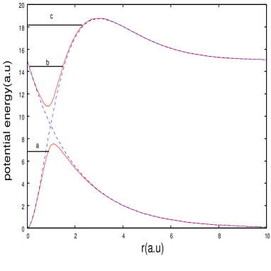
Figure 1: Broken lines: Diagonal elements of the potential matrix in Eq. (47). Solid lines: adiabatic potential energies. This system supports three resonances:  shape type (a) in channel 1, Feshbach type (b) and shape type (c) in channel 2.

Let us present an example of the perturbation theory for the two-threshold case. We revisit the 2-channel model potential with two thresholds that is taken up in Ref. sit-tol , i.e.

$$V(r)=\left(\begin{array}[]{cc}15e^{-0.5r}&5re^{-r}\\ 5re^{-r}&15(r^{2}-r-1)e^{-r}+15\end{array}\right).$$ (47)

The potential $V(r)$ supports three resonances. The adiabatic potential energy curve of the first channel supports one shape type resonance (a) while the other channel supports one Feshbach type (b) and one shape type (c) resonance. These resonances are depicted in Fig. 1. We carried out the diagonalization of the TSE, Eq. (11), using the discrete variable representation (DVR) functions as a basis set. The calculated resonance energies and widths with different numbers of the basis functions are given in Table 1. Let us call these results as direct numerical solutions. To implement perturbation calculations, we separate $V(r)$ into

$$V(r)=V_{0}(r)+V^{{}^{\prime}}(r)$$

where

$$V_{0}(r) = \left(\begin{array}[]{cc}15e^{-0.5r}&4re^{-r}\\ 4re^{-r}&15(r^{2}-r-1)e^{-r}+15\end{array}\right),$$

$$V^{{}^{\prime}}(r) = \left(\begin{array}[]{cc}0&re^{-r}\\ re^{-r}&0\end{array}\right).$$

We regard $V_{0}$ as the unperturbed potential energy and $V^{{}^{\prime}}$ as the perturbation potential energy. We calculate perturbation energies using the unperturbed solutions of TSE for the same box size $a=50$ as in Ref. sit-tol . Table 1 shows the results of first- and second-order perturbation calculations, and Figs. 2-4 depict how the numerical solutions converge in the complex plane. In the present model problem, the first-order resonance energy agrees with the direct numerical solutions to about 2 to 4 digits while the width agrees to about 2 to 3 digits. And the second-oder resonance energy agrees to about 3 to 5 digits while the width agrees to about 1 to 3 digits. An important fact which we must remark is that the resonance energy and width do not appear to converge in pace. For instance, the width of resonance “c” evaluated by the second-order perturbation theory appears less accurate than the first-order one while the resonance energy appears to have improved. The seeming deterioration of the width is a little overwhelming, all the more so for the improvement of the resonance energy. Nonetheless, the distance between the second-order result and the direct numerical one becomes rather small (see Fig. 4) in the complex plane, that is in the Siegert state perturbation theory the convergence is to be measured with respect to the variance

$$D=||E-\sum_{n}\lambda^{n}E^{(n)}||$$ (50)

rather than with respect to the real and imaginary parts of the sum, individually.

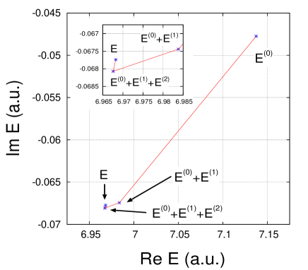
Figure 2: Complex energies for resonance a

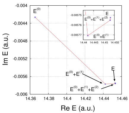
Figure 3: Complex energies for resonance b

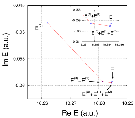
Figure 4: Complex energies for resonance c

Table 1: Columns $\Re$,. $\Im$, $D$, and $N$represent the real and imaginary parts of resonance energies, error variance in the complex plane, and the dimension of the DVR basis set, respectively.

		Resonance a				Resonance b				Resonance c
$N$		$\Re$	$\Im$	$D$		$\Re$	$\Im$	$D$		$\Re$	$\Im$	$D$
		$E^{(0)}$
100		7.13731291	$-$0.04777819	0.17022398		14.36514823	$-$0.00441589	0.08759123		18.25940438	$-$0.04709964	0.02402711
300		7.13739307	$-$0.04774929	0.17034758		14.36548638	$-$0.00426431	0.08762023		18.26200618	$-$0.04826379	0.02526594
500		7.13739307	$-$0.04774929	0.17034758		14.36548638	$-$0.00426431	0.08762023		18.26200618	$-$0.04826379	0.02526594
700		7.13739307	$-$0.04774929	0.17034758		14.36548638	$-$0.00426431	0.08762023		18.26200619	$-$0.04826379	0.02526594
		$E^{(0)}+E^{(1)}$
100		6.98368137	$-$0.06730063	0.01543038		14.44177638	$-$0.00607880	0.01094681		18.27770236	$-$0.05762106	0.00327772
300		6.98382603	$-$0.06744164	0.01560641		14.44219720	$-$0.00577079	0.01089678		18.28142974	$-$0.05926301	0.00330703
500		6.98382602	$-$0.06744165	0.01560641		14.44219720	$-$0.00577079	0.01089678		18.28142974	$-$0.05926301	0.00330703
700		6.98382603	$-$0.06744162	0.01560643		14.44219720	$-$0.00577079	0.01089678		18.28142974	$-$0.05926301	0.00330702
		$E^{(0)}+E^{(1)}+E^{(2)}$
100		6.96760487	$-$0.06783608	0.00067084		14.45258871	$-$0.00611007	0.00013451		18.28074487	$-$0.05788235	0.00031413
300		6.96755505	$-$0.06807440	0.00074684		14.45297412	$-$0.00575530	0.00011988		18.28452186	$-$0.05952953	0.00031773
500		6.96755905	$-$0.06807406	0.00074312		14.45297384	$-$0.00575631	0.00012019		18.28452397	$-$0.05952538	0.00031324
700		6.96756395	$-$0.06807313	0.00073832		14.45297366	$-$0.00575513	0.00012033		18.28452412	$-$0.05952393	0.00031208
		$E$ (Direct numerical solution)
100		6.96825547	$-$0.06767254			14.45272315	$-$0.00610584			18.28097965	$-$0.05767365
300		6.96822245	$-$0.06773922			14.45309397	$-$0.00575250			18.28473661	$-$0.05929537
500		6.96822245	$-$0.06773921			14.45309397	$-$0.00575250			18.28473661	$-$0.05929537
700		6.96822244	$-$0.06773923			14.45309397	$-$0.00575250			18.28473661	$-$0.05929536

IV CONCLUSIONS

In this paper we formulated one- and two-threshold SPSPT. The unusual orthonormality relationship of the SPSs results in somewhat nontrivial additional terms in SPSPT, and also it determines the phase of the perturbation wavefunction. In the degenerate threshold case, the one-threshold SPSPT formulas are obtained by appropriate scaling, and we also obtained an up-to-date correction to More’s theory. The numerical calculations show how the perturbation results converge. The convergence is achieved in the sense of the variance, Eq. 50, but not the resonance energy and width independently.

It is of interest to speculate on possible uses of SPSPT. One immediate application would be to the manipulation of Siegert poles. The shadow poles located near the physical sheet may be transformed to physical resonances by an appropriate perturbation. We leave issues such as this for a future task.

V ACKNOWLEDGMENT

We thank Dr. Tolstikhin for useful discussions. This work was supported in part by Grants-in-Aid for Scientific Research No. 15540381 from the Ministry of Education, Culture, Sports, Science and Technology, Japan, and also in part by the 21st Century COE program on “Innovation in Coherent Optical Science.”

Appendix A Consistency with orthonormality relationship and Siegert boundary condition in first order

Here, we prove that the first-order wavefunction satisfies the orthonormality relationship and the Siegert boundary condition consistently. First of all, we expand

$$\vec{c}_{n}^{T}\left(I_{N}+\frac{1}{\kappa_{n}+\kappa_{m}}B\right)\vec{c}_{m}=\delta_{mn},$$ (51)

into perturbation series, and compare both sides power by power for $\lambda$. The first-order equation shows

$$\vec{c}_{n}^{(0)T}\left(I_{N}-\frac{i}{k_{n}^{(0)}+k_{m}^{(0)}}B\right)\vec{c}_{m}^{(1)}+c_{n}^{(0)T}\frac{i(k_{n}^{(1)}+k_{m}^{(1)})}{(k_{n}^{(0)}+k_{m}^{(0)})^{2}}B\vec{c}_{m}^{(0)}$$

$$+\vec{c}_{n}^{(1)T}\left(I_{N}-\frac{i}{k_{n}^{(0)}+k_{m}^{(0)}}B\right)c_{m}^{(0)}=0.$$ (52)

And each term of the above equation reduces to

$$({\rm 1st~{}term}) = \sum_{l\neq m}^{2N}\frac{W^{{}^{\prime}}_{lm}\vec{c}_{n}^{(0)T}\vec{c}_{l}^{(0)}}{k_{l}^{(0)}(k_{n}^{(0)}+k_{m}^{(0)})}$$

$$+ \frac{2W^{{}^{\prime}}_{nm}}{(k_{n}^{(0)}+k_{m}^{(0)})(k_{m}^{(0)}-k_{n}^{(0)})}+\frac{W^{{}^{\prime}}_{mm}}{2k_{m}^{(0)2}}\delta_{nm},$$

$$({\rm 2nd~{}term})=\frac{W^{{}^{\prime}}_{nn}/k_{n}^{(0)}+W^{{}^{\prime}}_{mm}/k_{m}^{(0)}}{k_{n}^{(0)}+k_{m}^{(0)}}(\vec{c}_{n}^{(0)T}\vec{c}_{m}^{(0)}-\delta_{mn})$$

and

$$({\rm 3rd~{}term}) = \sum_{l\neq n}^{2N}\frac{W^{{}^{\prime}}_{ln}\vec{c}_{l}^{(0)T}\vec{c}_{m}^{(0)}}{k_{l}^{(0)}(k_{n}^{(0)}+k_{m}^{(0)})}$$

$$- \frac{2W^{{}^{\prime}}_{nm}}{(k_{n}^{(0)}+k_{m}^{(0)})(k_{m}^{(0)}-k_{n}^{(0)})}+\frac{W^{{}^{\prime}}_{nn}}{2k_{n}^{(0)2}}\delta_{nm}.$$

Hence, the left side of (52) reduces to

$$(\ref{eq:ortho-1st}) = \sum_{l=1}^{2N}\frac{W^{{}^{\prime}}_{lm}\vec{c}_{n}^{(0)T}\vec{c}_{l}^{(0)}}{k_{l}^{(0)}(k_{n}^{(0)}+k_{m}^{(0)})}+\sum_{l=1}^{2N}\frac{W^{{}^{\prime}}_{ln}\vec{c}_{l}^{(0)T}\vec{c}_{m}^{(0)}}{k_{l}^{(0)}(k_{n}^{(0)}+k_{m}^{(0)})}$$

$$+ \frac{W^{{}^{\prime}}_{mm}}{k_{m}^{(0)}}\left(\frac{1}{2k_{m}^{(0)}}-\frac{1}{k_{n}^{(0)}+k_{m}^{(0)}}\right)\delta_{mn}$$

$$+ \frac{W^{{}^{\prime}}_{mm}}{k_{m}^{(0)}}\left(\frac{1}{2k_{m}^{(0)}}-\frac{1}{k_{n}^{(0)}+k_{m}^{(0)}}\right)\delta_{mn}$$

$$= \frac{1}{k_{n}^{(0)}+k_{m}^{(0)}}\left(\sum_{l=1}^{2N}\frac{W^{{}^{\prime}}_{lm}\vec{c}_{n}^{(0)T}\vec{c}_{l}^{(0)}}{k_{l}^{(0)}}+\sum_{l=1}^{2N}\frac{W^{{}^{\prime}}_{ln}\vec{c}_{l}^{(0)T}\vec{c}_{m}^{(0)}}{k_{l}^{(0)}}\right).$$

By using a SPS sum rule,

$$\sum_{l=1}^{2N}\frac{1}{k_{l}^{(0)}}\vec{c}_{l}^{(0)}\vec{c}_{l}^{(0)T}=0,$$

we obtain

$$\sum_{l=1}^{2N}\frac{1}{k_{l}^{(0)}}W^{{}^{\prime}}_{lm}\vec{c}_{n}^{(0)T}\vec{c}_{l}^{(0)}=\vec{c}_{n}^{(0)T}\left(\sum_{l=1}^{2N}\frac{1}{k_{l}^{(0)}}c_{l}^{(0)}\vec{c}_{l}^{(0)T}\right)U^{{}^{\prime}}\vec{c}_{m}^{(0)}=0$$

and

$$\sum_{l=1}^{2N}\frac{1}{k_{l}^{(0)}}W^{{}^{\prime}}_{ln}\vec{c}_{l}^{(0)T}\vec{c}_{m}^{(0)} = \sum_{l=1}^{2N}\frac{1}{k_{l}^{(0)}}W^{{}^{\prime}}_{nl}\vec{c}_{l}^{(0)T}\vec{c}_{m}^{(0)}$$

$$= \vec{c}_{n}^{(0)T}U^{{}^{\prime}}\left(\sum_{l=1}^{2N}\frac{1}{k_{l}^{(0)}}\vec{c}_{l}^{(0)}\vec{c}_{l}^{(0)T}\right)\vec{c}_{m}^{(0)}=0.$$

Therefore, the first-order wavefunction is consistent with the orthonormality relationship.

Next, let us consider the Siegert boundary condition. We expand the Siegert boundary condition and compare both sides power by power for $\lambda$. The first-order equation shows

$$\left.\left(\frac{d}{dr}-ik_{n}^{(0)}\right)\phi_{n}^{(0)}-ik_{n}^{(1)}\phi_{n}^{(0)}\right|_{r=a}=0.$$

Then by using the coordinate representation of the SPS sum rule, namely

$$\sum_{l=1}^{2N}\frac{1}{k_{l}^{(0)}}\phi_{l}^{(0)}(r)\phi_{l}^{(0)}(r^{{}^{\prime}})=0,$$

we get

$$\left.\left(\frac{d}{dr}-ik_{n}^{(0)}\right)\phi_{n}^{(0)}\right|_{r=a} = \sum_{l\neq n}^{2N}\frac{W^{{}^{\prime}}_{ln}}{k_{l}^{(0)}(k_{n}^{(0)}-k_{l}^{(0)})}\left(\frac{d\phi_{l}^{(0)}}{dr}\right)_{r=a}$$

$$- k_{n}^{(0)}\sum_{l\neq n}^{2N}\frac{W^{{}^{\prime}}_{ln}}{k_{l}^{(0)}(k_{n}^{(0)}-k_{l}^{(0)})}\phi_{l}^{(0)}(a)$$

$$= -i\sum_{l\neq n}^{2N}\frac{1}{k_{l}^{(0)}}W^{{}^{\prime}}_{ln}\phi_{l}^{(0)}(a)$$

$$= -i\sum_{l=1}^{2N}\frac{1}{k_{l}^{(0)}}W^{{}^{\prime}}_{ln}\phi_{l}^{(0)}(a)+i\frac{W^{{}^{\prime}}_{nn}}{k_{n}^{(0)}}\phi_{n}^{(0)}(a)$$

$$= -i\int_{0}^{a}\left(\sum_{l=1}^{2N}\frac{1}{k_{l}^{(0)}}\phi_{l}^{(0)}(a)\phi_{l}^{(0)}\right)U^{{}^{\prime}}\phi_{n}^{(0)}dr$$

$$+ ik_{n}^{(1)}\phi_{n}^{(0)}(a)$$

$$= ik_{n}^{(1)}\phi_{n}^{(0)}(a)$$

Hence the first-order wavefunction is consistent with the Siegert boundary condition.

References

- (1) See, for instance, Chapter 8 in U. Fano and A. R. P. Rau, “Atomic Collisions and Spectra” (Academic Press, 1986, New York), and references therein.
- (2) A. J. F. Siegert, Phys. Rev. 56, 750 (1939).
- (3) O. I. Tolstikhin, V. N. Ostrovsky, and H. Nakamura, Phys Rev A58, 2077 (1998).
- (4) O. I. Tolstikhin, I. Yu. Tolstikhina, and C. Namba, Phys. Rev. A60, 4673 (1999).
- (5) S. Yoshida, S. Watanabe, C. O. Reinhold, and J. Burgdörfer, Phys. Rev. A60, 1113 (1999).
- (6) R. Santra, J. M. Shainline, and C. H. Greene, Phys. Rev. A71, 032703 (2005).
- (7) S. Tanabe, S. Watanabe, N. Sato, M. Matsuzawa, S. Yoshida, C. Reinhold, and J. Burgdörfer, Phys. Rev. A63, 052721 (2001).
- (8) G. V. Sitnikov and O. I. Tolstikhin, Phys. Rev. A67, 032714 (2003).
- (9) K. Toyota and S. Watanabe, Phys. Rev. A68, 062504 (2003).
- (10) R. M. More, Phys. Rev. A3, 1217 (1971).
- (11) R. M. More, Phys. Rev. A4, 1782 (1971).