Lagrangian dynamics of the Navier-Stokes equation

Abstract

Most researches on fluid dynamics are mostly dedicated to obtain the solutions of Navier-Stokes equation which governs fluid flow with particular boundary conditions and approximations. We propose an alternative approach to deal with fluid dynamics using the lagrangian. We attempt to develop a gauge invariant lagrangian which reconstructs the Navier-Stokes equation through the Euler-Lagrange equation. The lagrangian consists of gauge boson field ${\cal A}_{\mu}$ with appropriate content describing the fluid dynamics, i.e. ${\cal A}_{\mu}=(\Phi,-\vec{v})$. An example of applying the lagrangian to the interaction of fluid in a solitonic medium is also given.

^a) Geostech BPPT, Kompleks Puspiptek Serpong, Tangerang 15310, Indonesia
^b) Group for Theoretical and Computational Physics, Research Center for Physics, Indonesian Institute of Sciences, Kompleks Puspiptek Serpong, Tangerang 15310, Indonesia
^c) Department of Physics, University of Indonesia, Kampus UI Depok, Depok 16424, Indonesia

1 Introduction

The fluid dynamics still remains as an unsolved problem. Mathematically, a fluid flow is described by the Navier-Stokes (NS) equation [1]:

$$\frac{\partial\vec{v}}{\partial t}+(\vec{v}\cdot\vec{\triangledown})\vec{v}=-\frac{1}{\rho}\vec{\triangledown}P-\mu\vec{\triangledown}^{2}\vec{v}\;,$$ (1)

where $\vec{v}$ is fluid velocity, $P$ is pressure, $\rho$ is density and $\mu$ is the coefficient of viscosity.

In principle, the study of fluid dynamics is focused on solving the Navier-Stokes equation with particular boundary conditions and / or some approximations depend on the phenomenon under consideration. Mathematically it has been known as the boundary value problem. The most difficult problem in fluid dynamics is turbulence phenomenon. In the turbulence regime, the solution for the Navier-Stoke equation has a lot of Fourier modes, such that the solution is untrackable numerically or analytically. It is predicted that the strong turbulence has $10^{10}$ numerical operation [2]. This motivates us to look for another approach rather than the conventional ones. This paper treats the fluid dynamics differently than the conventional point of view as seen in some fluid dynamics textbooks. In this approach, the fluid is described as a field of fluid buch. We use the gauge field theory to construct a lagrangian describing fluid dynamics by borrowing the gauge principle. The Navier-Stoke equation can be obtained from this Lagrangian as its equation of motion through the Euler-Lagrange principles.

2 Maxwell-like equation for ideal fluid

The abelian gauge theory $U(1)$ is an electromagnetic theory that reproduces the Maxwell equation. To build a lagrangian that is similar with the abelian gauge theory, we should ’derive’ the Maxwell-like equation from the Navier-Stokes equation [3]. The result can be used as a clue to construct a lagrangianan for fluid that satisfies gauge principle. Considering the Navier-Stokes equation Eq. (1) for an ideal and incompressible fluid,

$$\rho\left(\frac{\partial\vec{v}}{\partial t}+(\vec{v}.\vec{\triangledown})\vec{v}\right) = -\vec{\triangledown}P\;,$$ (2)

$$\vec{\triangledown}\cdot\vec{v} = 0\;.$$ (3)

Using the identity $\vec{v}\times(\vec{\triangledown}\times\vec{v})=\vec{\triangledown}(\frac{1}{2}\vec{v}^{2})-(\vec{v}\cdot\vec{\triangledown})\vec{v}$, it can be rewritten as,

$$\frac{\partial\vec{v}}{\partial t}+\vec{\triangledown}\left(\frac{1}{2}\vec{v}^{2}\right)-\vec{v}\times(\vec{\triangledown}\times\vec{v})=-\frac{1}{\rho}\vec{\triangledown}P\;,$$ (4)

and then,

$$\frac{\partial\vec{v}}{\partial t}=\vec{v}\times(\vec{\triangledown}\times\vec{v})-\vec{\triangledown}\left(\frac{1}{2}\vec{v}^{2}+\frac{P}{\rho}\right)\;.$$ (5)

Putting the scalar potenstial $\Phi=\frac{1}{2}\vec{v}^{2}+\frac{P}{\rho}$ , the vorticity $\vec{\omega}=\vec{\triangledown}\times\vec{v}$ and the Lamb’s vector $\vec{l}=\vec{\omega}\times\vec{v}$, the equation becomes,

$$\frac{\partial\vec{v}}{\partial t} = -\vec{\omega}\times\vec{v}-\vec{\triangledown}\Phi$$ (6)

$$= -\vec{l}-\vec{\triangledown}\Phi\;.$$

Imposing curl operation in Eq. (6) we obtain the vorticity equation as follow,

$$\frac{\partial\vec{\omega}}{\partial t}=-\vec{\triangledown}\times(\vec{\omega}\times\vec{v})\;.$$ (7)

In order to get the Maxwell-like equation for an ideal fluid, let us take divergence operation for Eq. (6), that is

$$\frac{\partial}{\partial t}(\vec{\triangledown}\cdot\vec{v}) = -\vec{\triangledown}\cdot\vec{l}-\vec{\triangledown}^{2}\Phi$$

$$\vec{\triangledown}\cdot\vec{l}=-\vec{\triangledown}^{2}\Phi = \tilde{\rho}\;.$$ (8)

Here we have used the incompressible condition, while by definition the divergence of vorticity is always zero, i.e. $\vec{\triangledown}\cdot\vec{\omega}=0$. Imposing again curl operation, we have,

$$\frac{\partial}{\partial t}(\vec{\triangledown}\times\vec{v}) = -\vec{\triangledown}\times\vec{l}-\vec{\triangledown}\times(\vec{\triangledown}\Phi)\;,$$

$$\frac{\partial\vec{\omega}}{\partial t} = -\vec{\triangledown}\times\vec{l}\;,$$ (9)

$$\vec{\triangledown}\times\vec{l} = -\frac{\partial\vec{\omega}}{\partial t}\;,$$

using the identity $\vec{\triangledown}\times(\vec{\triangledown}\cdot\phi)=0$.

Now, let us consider the definition of the Lamb’s vector $\vec{l}=\vec{\omega}\times\vec{v}$. Taking the derivative ${\partial}/{\partial t}$ in the definition we obtain,

$$\frac{\partial\vec{l}}{\partial t}=\frac{\partial\vec{\omega}}{\partial t}\times\vec{v}+\vec{\omega}\times\frac{\partial\vec{v}}{\partial t}\;.$$ (10)

Substituting Eq. (6) and (7), we get,

$$\vec{\triangledown}\times\vec{\omega}=\alpha\vec{j}+\alpha\frac{\partial\vec{l}}{\partial t}\;,$$ (11)

where,

$$\alpha = \frac{1}{\vec{v}^{2}}\;,$$ (12)

$$\vec{j} = -\vec{v}\vec{\triangledown}^{2}\Phi+\left[\vec{\triangledown}\times(\vec{v}\cdot\vec{\omega})\right]\vec{v}+\vec{\omega}\times\vec{\triangledown}(\Phi+\vec{v}^{2})+2\left[(\vec{\triangledown}\times\vec{v})\cdot\vec{\triangledown}\right]\vec{v}\;.$$ (13)

These results induce a series of equations,

$$\vec{\triangledown}\cdot\vec{l} = \tilde{\rho}\;,$$ (14)

$$\vec{\triangledown}\times\vec{l} = -\frac{\partial\vec{\omega}}{\partial t}\;,$$ (15)

$$\vec{\triangledown}\cdot\vec{\omega} = 0\;,$$ (16)

$$\vec{\triangledown}\times\vec{\omega} = \alpha\vec{j}+\alpha\frac{\partial\vec{l}}{\partial t}\;,$$ (17)

that is clearly the Maxwell-like equation for fluids. If the fluid velocity is time independent, then $\vec{l}=-\vec{\triangledown}\Phi$. This is the ”electrostatic” condition. We use these results to develop gauge field theory approach for fluid dynamics in the next section.

3 Bosonic lagrangian for fluid

The correspondences of the electromagnetism and the ideal fluid can be written as follow,

$$\overrightarrow{B} \leftrightarrow \overrightarrow{\omega}\;,$$

$$\overrightarrow{E} \leftrightarrow \overrightarrow{l}\;,$$ (18)

$$\overrightarrow{A} \leftrightarrow \overrightarrow{\vec{v}}\;,$$

$$\phi \leftrightarrow \Phi\;,$$

where $\overrightarrow{B}$ is the magnetic field, $\overrightarrow{E}$ is the electric field, $\overrightarrow{A}$ is the electromagnetics vector, $\phi$ is a scalar function, $\overrightarrow{\omega}$ is the fluid vorticity, $\overrightarrow{l}$ is the Lamb’s vector, $\vec{v}$ is fluid velocity and $\Phi$ is the scalar potential. The same as the electromagnetics field, we have a four vector $A_{\mu}=(\phi,\vec{A})$ which can be interpreted as the four vector for fluid dynamics, ${\cal A}_{\mu}=(\Phi,-\vec{v})$. In the electromagnetics field, the scalar and vector potentials, $\phi$ and $\vec{A}$, are auxiliary fields. On the other hand, in the fluid dynamics the scalar potential $\Phi=\frac{1}{2}\vec{v}^{2}+V$ describes the kinetic energy of fluid, while the vector potential $\vec{v}$ is fluid velocity. Similar to the electromagnetics field, the lagrangian density has the form of [4],

$${\cal L}_{NS}=-\frac{1}{4}F_{\mu\nu}F^{\mu\nu}+g{\cal J}_{\mu}{\cal A}^{\mu}\;,$$ (19)

where,

$${\cal F}_{\mu\nu}\equiv\partial_{\mu}{\cal A}_{\nu}-\partial_{\nu}{\cal A}_{\mu}\;.$$ (20)

This Lagrangian obeys the gauge principles, i.e. it is invariant under a particular local gauge transformation,

$${\cal A}_{\mu}\rightarrow{\cal A}_{\mu}^{\prime}\equiv A_{\mu}+\frac{1}{g}\partial_{\mu}\theta\;,$$ (21)

where $\theta=\theta(x)$ is an arbitrary real constant. It is easy to show that the lagrangian density in Eq. (19) is invariant under this transformation.

The equation of motion governed by this lagrangian can be derived using the Euler-lagrange equation in term of ${\cal A}_{\mu}$,

$$\partial^{\nu}\frac{\partial{\cal L}_{NS}}{\partial(\partial^{\nu}{\cal A}^{\mu})}-\frac{\partial{\cal L}_{NS}}{\partial{\cal A}^{\mu}}=0\;.$$ (22)

After a straightforward calculation, we obtain,

$$\partial^{\nu}(\partial_{\mu}{\cal A}_{\nu}-\partial^{\nu}\partial_{\nu}{\cal A}_{\mu})-g{\cal J}_{\mu}=0\;.$$ (23)

Now integrating it over $x^{\nu}$ and considering only the non-trivial relation as $\nu\neq\mu$ gives,

$$\partial_{0}A_{i}-\partial_{i}A_{0}=-g\oint\mathrm{d}x_{0}J_{i}=g\oint\mathrm{d}x_{i}J_{0}\;.$$ (24)

Since $A_{i}=-\vec{v}$, $A_{o}=\Phi$, $\partial_{o}={\partial}/{\partial t}$ and $\partial_{i}=\vec{\triangledown}$. we have,

$$-\frac{\partial\vec{v}}{\partial t}-\vec{\triangledown}\Phi=-g\vec{\tilde{J}}\;,$$ (25)

where $\tilde{J}_{i}\equiv\oint\mathrm{d}x_{0}J_{i}=-\oint\mathrm{d}x_{i}J_{0}$. Concerning the scalar potential given by $\Phi=\frac{1}{2}\vec{v}^{2}+V$, we obtain,

$$-\frac{\partial\vec{v}}{\partial t}-\frac{1}{2}\vec{\triangledown}\left|\vec{v}\right|^{2}-\vec{\triangledown}V=-g\vec{\tilde{J}}\;.$$ (26)

Borrowing the identity $\frac{1}{2}\vec{\triangledown}\left|\vec{v}\right|^{2}=(\vec{v}\cdot\vec{\triangledown})\vec{v}+\vec{v}\times(\vec{\triangledown}\times\vec{v})$, we get,

$$\frac{\partial\vec{v}}{\partial t}+(\vec{v}\cdot\vec{\triangledown})\vec{v}=-\vec{\triangledown}V-\vec{v}\times\vec{\omega}-g\vec{\tilde{J}}\;,$$ (27)

where $\vec{\omega}\equiv\vec{\triangledown}\times\vec{v}$ is the vorticity. This result reproduces the general NS equation with arbitrary conservative forces ($\vec{\triangledown}V$). The potential $V$ can be associated with some known forces, for example, ${P}/{\rho}$, ${(Gm)}/{r}$ and $\eta(\vec{\triangledown}\cdot\vec{v})$. Here, $P,\rho,G,\nu+\eta$ denote pressure, density, gravitational constant and viscosity as well.

4 Interaction between soliton and fluid

In this section we describe an idea to apply the theory described in the preceeding section. We give an example on applying the theory to provide a consistent way for the interaction between soliton and fluid system. Soliton is a pulse-like nonlinear wave which forms a collision with similar pulse having unchanged shape and speed [9]. The wave equations that exhibit soliton are the KdV equation, the Nonlinear Schrodinger equation, the Sine-Gordon equation, Nonlinear Klein-Gordon equation, the Born-Infeld equation, the Burger equation and the Boussiness equation. Considering the Nonlinear Klein-Gordon as follow:

$$\frac{\partial^{2}\phi}{\partial t^{2}}-\frac{\partial^{2}\phi}{\partial x^{2}}-m^{2}\phi+\frac{\lambda}{3!}\phi^{3}=0\;.$$ (28)

The equation is a continuum version of that describes a propagation of molecular vibration (vibron) in $\alpha-$helical protein [8]. The vibration excitation in the $\alpha-$helix protein propagates from one group to the next because of the dipole-dipole interaction between the group. The wave is called the Davidov soliton [8]. Davydov has shown that in $\alpha-$helical protein soliton can be formed by coupling the propagation of amide$-I$ vibrations with longitudinal phonons along spines and that such entities are responsible for mechanism of energy transfer in biological system [8]. If $\alpha-$helical protein immersed in Bio-fluid, then the phenomenon can be described by the interaction of soliton with fluid system. In standard technique in fluid dynamics, the problem will be done by solving of the Navier-Stokes equation and nonlinear Klein-Gordon simultaneously.

In our current approach the problem is treated as follow. First, let us rewrite Eq. (28) into four vector formalism,

$$\partial_{\mu}\partial^{\mu}\phi-m^{2}\phi+\frac{\lambda}{3}\phi^{3}=0\;.$$ (29)

Using the Euler-Lagrange equation, the lagrangian density is,

$${\cal L}=\frac{1}{2}(\partial_{\mu}\phi)(\partial^{\mu}\phi)+\frac{m^{2}}{2!}\phi^{2}-\frac{\lambda}{4!}\phi^{4}\;.$$ (30)

In order to couple this lagrangian with the Navier-Stoke lagrangian in Eq. (19), it is sufficient to replace the covariant derivative in Eq. (30) [4],

$${\cal D}_{\mu}\phi=(\partial_{\mu}+ig{\cal A}_{\mu})\phi\;.$$ (31)

The covariant derivative is invariant under local gauge transformation[6]. Then the interaction between soliton and fluid system obeys the lagrangian,

$${\cal L}=-\frac{1}{4}{\cal F}_{\mu\nu}{\cal F}^{\mu\nu}+\frac{1}{2}({\cal D}_{\mu}\phi)({\cal D}^{\mu}\phi)+\frac{m^{2}}{2}\phi^{2}-\frac{\lambda}{4!}\phi^{4}\;.$$ (32)

One interesting case is when we consider a static condition, i.e. $\partial_{t}f=0$ with $f$ is an arbitrary functions. Substituting ${\cal A}_{\mu}=(\Phi,-\vec{v})$ into Eq. (32) then the Lagrange density becomes,

$${\cal L}=-\frac{1}{2}(\nabla\times\vec{v})^{2}+\frac{1}{2}|(\nabla-ig\vec{v})\phi|^{2}+\frac{m^{2}}{2!}\phi^{2}-\frac{\lambda}{4!}\phi^{4}\;.$$ (33)

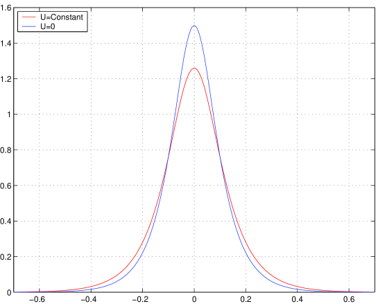
Figure 1: Single soliton solution of the nonlinear Klein-Gordon equation.

The lagrangian is nothing else similar with the Ginzburg-Landau free energy lagrangian that is widely used in superconductor theory [7]. We have seen that the phenomenon of $\alpha-$helical protein immersed in fluid similar with quantum electrodynamics for boson particle, while for static case it is similar with the Ginzburg-Landau model for superconductor.

In order to perform an explicit calculation, suppose we have one-dimensional velocity in $x$ direction $\vec{v}=(u(x),0,0)$ and $\phi=\phi(x)$. Then the lagrangian in Eq.(33) reads,

$${\cal L}=\frac{1}{2}\phi_{x}^{2}-\frac{1}{2}g^{2}u^{2}\phi^{2}+\frac{m^{2}}{2!}\phi^{2}-\frac{\lambda}{4!}\phi^{4}\;.$$ (34)

Substituting it into Euler-lagrangian equation we arrive at,

$$\frac{d^{2}\phi}{dx^{2}}-\gamma(x)\phi+\frac{\lambda}{3!}\phi^{3}=0\;,$$ (35)

where $\gamma(x)=m^{2}-g^{2}u(x)^{2}$. The equation is called the variable coefficient of nonlinear Klein-Gordon equation.

Further, we can consider a special case when the fluid velocity is constant, $u(x)=U$, to obtain

$$\frac{d^{2}\phi}{dx^{2}}-\gamma\phi+\alpha\phi^{3}=0\;,$$ (36)

with $\gamma=m^{2}-g^{2}U^{2}$ and $\alpha={\lambda}/{3!}$. To solve the equation, we can use a mathematical trick as follows. First multiply it by ${d\phi}/{dx}$,

$$\frac{d\phi}{dx}\frac{d^{2}\phi}{dx^{2}}-\gamma\phi\frac{d\phi}{dx}+\alpha\phi^{3}\frac{d\phi}{dx}=0\;,$$ (37)

then integrating out over $x$ and putting the integration constant as zero due to integrable condition $\lim_{x\rightarrow\pm\infty}\phi=0$. Finally we obtain,

$$\left(\frac{d\phi}{dx}\right)^{2}-\gamma\phi^{2}+\frac{\alpha}{2}\phi^{4}=0\;,$$ (38)

and it can be rewritten further as,

$$\int\frac{d\phi}{\phi(\delta^{2}-\phi^{2})^{\frac{1}{2}}}=\int\sqrt{\frac{\alpha}{2}}dx\;,$$ (39)

where $\delta^{2}={2\gamma}/{\alpha}$. Integration of the left hand side and solving the equation for $\phi$ provide the result,

$$\phi = \frac{2\delta e^{-\sqrt{\frac{\alpha}{2}}\delta x}}{1+e^{-2\sqrt{\frac{\alpha}{2}}\delta x}}=\frac{2\delta}{e^{\sqrt{\frac{\alpha}{2}}\delta x}+e^{-\sqrt{\frac{\alpha}{2}}\delta x}}$$ (40)

$$= \frac{\delta}{\cosh(\sqrt{\frac{\alpha}{2}}\delta x)}0=\delta\mathrm{sech}(\sqrt{\frac{\alpha}{2}}\delta x)\;.$$

Thus, the solution for a homogeneous nonlinear Klein - Gordon equation is,

$$\phi(x)=A\mathrm{sech}(\Lambda x)\;,$$ (41)

where $A={(12\gamma)}/{\lambda}$ and $\Lambda={(12\sqrt{3}\gamma)}/{\lambda^{3/2}}$. This result is depicted in Fig. 1. The figure shows that the soliton propagation will be damped by fluid. This theory also can be applied in turbulence phenomenon [3].

5 Conclusion

We have shown an analogy between electromagnetics field and fluid dynamics using the Maxwell-like equation for an ideal fluid. The results provide a clue that we might be able to build a gauge invariant lagrangian density, the so-called Navier-Stokes lagrangian in term of scalar and vector potentials ${\cal A}_{\mu}$. Then the Navier-Stokes equation is obtained as its equation of motion through the Euler-lagrange principle. The application of the theory is wide, for instance the interaction between Davydov soliton with fluid system that can be described by the lagrangian density which is similar to quantum electrodynamics for boson particle. In the static condition, the lagrangian density is similar with the Ginzburg-Landau lagrangian. If the fluid flow is parallel with soliton propagation we also obtain the variable coefficient Nonlinear Klein-Gordon equation. Single soliton solution has been obtained in term of a second hyperbolic function. The result showed that the present fluid flow will give a damping in solitary wave propagation.

References

- [1] P. Kundu (1996), Fluids Mechanics, Addison-Wesley, New York.
- [2] T. Mulin (1995), The Nature of Chaos, Clarendon Press, Oxford.
- [3] A. Sulaiman (2005), Contruction of The Navier-Stokes Equation using Gauge Field Theory Approach, Master Theses at Department of Physics, University of Indonesia.
- [4] A. Sulaiman and L.T. Handoko (2005), Gauge field theory approach to construct the Navier-Stokes equation, arXiv:physics/0508086.
- [5] Huang.K (1992), Quarks, Leptons and Gauge Fields, Worlds Sceintific, Singapore.
- [6] Muta.T (2000), Foundation of Quantum Chromodynamics, Worlds Sceintific, Singapore.
- [7] Binney. J.J et.al. (1995), The Theory of Critical Phenomena, Clarendon press, Oxford.
- [8] Takeno, S (1987), Vibron Soliton and Coherent Polarization, Collected paper Dedicated to prof K Tomita, Editor:Takeno.S et al , Kyoto University Press. Kyoto.
- [9] A. Scott, et al (1973), Soliton: A New Concepts in Applied Science,Proceeding of the IEEE, 61, 1443-1464.