Geometry Optimization of Crystals by the Quasi-
Independent Curvilinear Coordinate Approximation

Abstract

The quasi-independent curvilinear coordinate approximation (QUICCA) method [K. Németh and M. Challacombe, J. Chem. Phys. 121, 2877, (2004)] is extended to the optimization of crystal structures. We demonstrate that QUICCA is valid under periodic boundary conditions, enabling simultaneous relaxation of the lattice and atomic coordinates, as illustrated by tight optimization of polyethylene, hexagonal boron-nitride, a (10,0) carbon-nanotube, hexagonal ice, quartz and sulfur at the $\Gamma$-point RPBE/STO-3G level of theory.

I Introduction

Internal coordinates, involving bond stretches, angle bends, torsions and out of plane bends, etc. are now routinely used in the optimization of molecular structures by most standard quantum chemistry programs. Internal coordinates are advantageous for geometry optimization as they exhibit a reduced harmonic and anharmonic vibrational coupling Pulay (1969); Pulay et al. (1979); Fogarasi et al. (1992); H. F. Schaefer III (1977). This effect allows for larger steps during optimization, reducing the number of steps by 7-10 times for small to medium sized molecules, relative to Cartesian conjugate gradient schemes Bučko et al. (2005).

Recently, Kudin, Scuseria and Schlegel (KSS) Kudin et al. (2001) and Andzelm, King-Smith and Fitzgerald (AKF) Andzelm et al. (2001) reported the first crystal structure optimizations using internal coordinates. These authors proposed new ways of building Wilson’s B matrix Wilson et al. (1955) under periodic boundary conditions. The B-matrix (and its higher order generalizations), defines the transformation between energy derivatives in Cartesian coordinates and those in internal coordinates Wilson et al. (1955); Challacombe and Cioslowski (1991). The scheme presented by KSS allows the simultaneous relaxation of atomic positions and lattice parameters, while the method developed by AKF allows relaxation of atomic positions with a fixed lattice.

More recently still, Bučko, Hafner and Ángyán (BHA) Bučko et al. (2005) presented a more “democratic” formulation of Wilson’s B matrix for crystals, realizing that changes in periodic internal coordinates may have non-vanishing contributions to the lattice. The BHA definition of the B-matrix will be used throughout this paper.

In the present article, we extend our recently developed optimization algorithm, the Quasi Independent Curvilinear Coordinate Approach (QUICCA) Németh and Challacombe (2004) to the condensed phase. QUICCA is based on the idea that optimization can be carried out in an uncoupled internal coordinate representation, with coupling effects accounted for implicitly through a weighted fit. So far, QUICCA has been simple to implement, robust and efficient for isolated molecules, with a computational cost that scales linearly with system size. However, nothing is yet known about the applicability of QUICCA for crystals. In crystals, coupling may be very different from that encountered in isolated molecules, and there may be significant effects from changes in the lattice. If QUICCA also works well for crystals, then it presents a viable offshoot of gradient only algorithms for the large scale optimization of atomistic systems.

In the following, we first review the construction of Wilson’s B matrix for crystals (Sec. II.1), and then in Sec. III we go over the QUICCA algorithm and discuss its implementation for periodic systems. In Sec. IV, results of test calculations ranging over a broad class of crystalline systems are presented. We discuss these results in Sec. V, and then go on to present our conclusions in Sec. VI.

II Methodology

II.1 Wilson’s B matrix for crystals

In this section we briefly review the BHA approach to construction of the periodic B-matrix, with a somewhat simplified notation. A more detailed discussion can be found in Ref. [Bučko et al., 2005] and a background gained from Wilson’s book, Ref. [Wilson et al., 1955].

The independent geometrical variables of a crystal are the fractional coordinates $\vec{f}_{k}$, and the lattice vectors $\vec{h}_{l}$. The absolute Cartesian position of the $k$-th atom, $\vec{r}_{k}$, is related to the corresponding fractional coordinates by

$$\vec{r}_{k}={\bf h}\vec{f}_{k},$$ (1)

where ${\bf h}=\{\vec{h}_{1}:\vec{h}_{2}:\vec{h}_{3}\}$ is the matrix of (coloumn wise) Cartesian lattice vectors.

The periodic B-matrix is naturally coloumn blocked, with a fractional coordinate block ${\bf B}^{f}_{\scriptscriptstyle N_{i}\times 3N_{a}}$, and a lattice coordinate block ${\bf B}^{h}_{\scriptscriptstyle N_{i}\times 9}$. The full B-matrix is then ${\bf B}=\left({\bf B}^{f}:{\bf B}^{h}\right)$, a $N_{i}\times(3N_{a}+9)$ matrix with $N_{i}$ the number of internal coordinates and $N_{a}$ the number of atoms. Elements of ${\bf B}^{f}$ involve total derivatives of internal coordinates with respect to fractionals,

$$\vec{b}_{ik}=\frac{d\phi_{i}}{d\vec{f}_{k}},\qquad k=1,N_{a}\,,$$ (2)

where $\phi_{i}$ is the $i$-th internal coordinate and the B-matrix elements are atom-blocked as the three-vector $\vec{b}_{ik}$. Only the atoms $k$ that determine internal coordinate $i$ are non-zero, making ${\bf B}^{f}$ extremely sparse. Conventional elements of Wilson’s B-matrix, $\frac{\partial\phi_{i}}{\partial\vec{r}_{k}}$, are related to these total derivatives by the chain rule:

$$\vec{b}_{ik}=\frac{d\phi_{i}}{d\vec{f}_{k}}=\frac{\partial\phi_{i}}{\partial\vec{r}_{k}}{\mathbb{h}}.$$ (3)

Likewise, elements of ${\bf B}^{h}$ are

$$\vec{b}_{il}=\frac{d\phi_{i}}{dh_{l}}=\sum_{m\in{\bf n}_{i}}\frac{\partial\phi_{i}}{\partial\vec{r}_{m}}f_{ml},\qquad l=1,3$$ (4)

where $f_{ml}$ is the $l$-th component of the fractional coordinate corresponding to atom $m$, and the summation goes over the set ${\bf n}_{i}$ of all atoms that determine $\phi_{i}$, i.e. in case of torsions and out of plane bendings, there are four atoms in this set. From Eq. (4), it is clear that change in the lattice has the potential to change each internal coordinate, through the fractionals and depending on symmetry, so that in general we can expect ${\bf B}^{h}$ to be dense. Also, note that $f_{ml}$ can be greater then $1$ if atom $m$ is not in the central cell.

II.2 Internal Coordinate Transformations

With the B-matrix properly defined, transformation of Cartesian coordinates, lattice vectors and their corresponding gradients into internal coordinates remains. As in the case of the B-matrix, the Cartesian gradients are partitioned into a fractional component,

$$\vec{g}^{\,f}_{k}=\frac{dE}{d\vec{f}_{k}}=\frac{\partial E}{\partial\vec{r}_{k}}{\bf h},\qquad k=1,N_{a}\,,$$ (5)

and a lattice component, $\vec{g}^{h}$, with 9 entries involving the total derivatives $\frac{dE}{d\vec{h}_{l}}$; the emphasis underscores the fact that some programs produce partial derivatives with respect to lattice vectors, and this subtly must be taken into account (e.g. see Eq. (9) in Ref. [Bučko et al., 2005]).

With this blocking structure, gradients in internal coordinates are then defined implicitly by the equation

$$\vec{g}^{\,i}\left({\bf B}^{f}:{\bf B}^{h}\right)=\left(\vec{g}^{\,f}:\vec{g}^{\,h}\right)\;,$$ (6)

which may be solved in linear scaling CPU time, through Cholesky factorization of the matrix ${\bf B}^{t}{\bf B}$ that enters the left-handed pseudo-inverse, followed by forward and backward substitution, as described in Ref. [Németh et al., 2000]. Linear scaling factorization of ${\bf B}^{t}\bf B$ may be achieved, as the upper left-hand $3N_{a}\times 3N_{a}$ block is hyper-sparse, leading also to a hyper-sparse elimination tree and sparse Cholesky factors, similar to the case of isolated molecules Németh et al. (2000). Note however that the factorization of ${\bf BB}^{t}$, involved in construction of a right-handed pseudo-inverse, has the dense $9\times N_{i}$ row uppermost and the dense $N_{i}\times 9$ coloumn foremost, leading to dense Cholesky factors. Thus, the left- and right-handed approach are not equivalent for internal coordinate transformations of large crystal systems, as they are in the case of gas phase molecules, when using sparse linear algebra to achieve a reduced computational cost.

Once predictions are made for improved values of internal coordinates, based on the internal coordinates and their gradients, new Cartesian coordinates are calculated via an iterative back-transformation as described in Ref. [Németh and Challacombe, 2004], which also scales linearly with the system-size. At each step of the iterative back-transformation, fractional coordinates and lattice vectors are updated and the corresponding atomic Cartesian coordinates are computed. From these, updated values of the internal coordinates are found, and the next iteration is started. Besides these minor details, the back-transformation is the same as that used for isolated molecules.

III Implementation

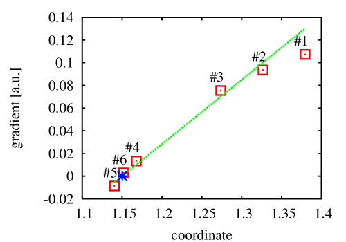
Figure 1: Progression of RHF-MIC/STO-3G gradients for a hydrogen bond coordinate in hexagonal ice, starting from the crystal structure Goto et al. (1990). Numbers label QUICCA optimization steps, and the star shows the predicted minimum given by a weighted line fit (dashed line) of the previous 6 points.

III.1 The QUICCA algorithm for crystals

Details of the QUasi-Independent Curvilinear Coordinate Approximation (QUICCA) for geometry optimization of isolated molecules have been given in Ref. [Németh and Challacombe, 2004]. Here we provide a brief overview of the method.

QUICCA is based on the trends shown by internal coordinate gradients during geometry optimization. See Fig. 1 for example. These trends can be exploited by a weighted curve fit for each internal coordinate gradient, allowing an independent, one-dimensional extrapolation to zero. The predicted minima for each internal coordinate collectively determines one optimization step. This method works surprisingly well, but only when the weights are chosen to account for coupling effects; when coupling is strong, the weights should be small and vica versa. Also, the fitting process has an important averaging effect on coupling that contributes to the success of QUICCA.

The only difference in our current implementation of QUICCA, relative to that described in Ref. [Németh and Challacombe, 2004], is that merging the connectivities from recent optimization steps is no longer carried out. Omitting this connectivity merger does not change the results for Baker’s test suite as given in Ref. [Németh and Challacombe, 2004], and does not appear to diminish the overall effectiveness of QUICCA.

III.2 The periodic internal coordinate system

In setting up a periodic internal coordinate system, it is first important to consider the situation where, during optimization, atoms wrapping across cell boundaries lead to large (unphysical) jumps in bond lengths, angles, etc. This situation is avoided here by employing a minimum image criterion to generate a set of Cartesian coordinates consistent with a fixed reference geometry.

Also, because internal coordinates span cell boundaries, it is convenient to work with a $3\times 3\times 3$ supercell, including the central cell surrounded by its 27 nearest neighbors. Even though a smaller replica of 8 cells, with lattice indices between $0$ and $1$ contains all necessary local internal coordinates, we prefer to employ the larger supercell, to avoid fragmentation of bonds etc at the cell boundaries. Then, all internal coordinates are identified in the supercell by means of a recognition algorithm, just as for isolated molecules. Finally, internal coordinates are discarded that do not involve at least one atom in the central cell.

This procedure produces symmetry equivalent internal coordinates, among those internal coordinates that cross cell boundaries. In the present implementation these equivalent coordinates are not filtered out, since their presence has no major effect on the optimization; the equivalent coordinates result in exactly the same line fit and same predicted minima.

It is worth noting that an appropriate internal coordinate recognition scheme is extremely important to the success of internal coordinate optimization. Here, we are using a still experimental algorithm, which we hope to describe in a forthcoming paper.

III.3 Treatment of constraints

In the treatment of constraints, we distinguish between soft and hard constraints. Soft constraints approach their target value as the optimization proceeds, reaching it at convergence. Most internal coordinate constraints are of the soft type in our implementation. The application of soft constraints is particularly useful in situations where it is difficult to construct corresponding Cartesian coordinates that satisfy the constrained values. Hard constraints are set to their required value at the beginning and keep their value during the optimization. Cartesian and lattice constraints are hard constraints in the current implementation.

Our method of treating hard constraints is similar to Baker’s projection scheme Baker et al. (1996); columns of the B-matrix corresponding to hard constraints are simply zeroed. This zeroing reflects the simple fact that a constrained Cartesian coordinate or lattice parameter may not vary any internal coordinate. Note, that if the lattice parameters $a,b,c,\alpha,\beta$ and $\gamma$ are constrained, ${\bf B}^{h}$ must be transformed from a lattice-vector representation into a lattice-parameter representation by using the generalized inverse of the lattice-parameter Jacobian. This transformation results in 6 columns corresponding to the 6 lattice parameters. After zeroing the relevant columns, this portion of the ${\bf B}^{h}$ matrix is transformed back into the original $N_{i}\times 9$ representation. In addition, this approach guarantees that during the iterative back-transformation no displacements occur for constrained coordinates or parameters.

In both cases, it is necessary to project out the constraint-space component of the Cartesian gradients, so that the internal coordinate gradients remain consistent with the constrained internal coordinates. As recommended by Pulay H. F. Schaefer III (1977), this is accomplished via projection;

$$\vec{g}\;^{\prime}={\bf P}\vec{g}\,,$$ (7)

where $\bf P$ is the purification projector that filters out the constraint-space. For Cartesian variables, this together the aforementioned zeroing of ${\bf B}^{f}$ is sufficient to enforce a hard constraint. For constrained internal coordinate variables though, this projection is not entirely sufficient, as there are further contaminants that can arise in the left-handed pseudo-inverse transformation to internal coordinates. These contaminants can be rigorously removed by introducing a further projection in the transformation step, as suggested by Baker Baker et al. (1996). However, toward convergence these contaminants disappear, and in practice, we find good performance without introducing an additional purification step. And so, Eq. (7) is the only purification used in the current implementation, for both hard and soft constraints.

While purification of the gradients is sufficient for the already satisfied hard constraints, the soft internal coordinate constraints must be imposed at each geometry step. This is accomplished through setting the constrained and optimized internal coordinates, followed by iterative back transformation to Cartesian coordinates. This procedure finds a closest fit that satisfies the modified internal coordinate system, as described in Refs. [H. F. Schaefer III, 1977] and [Németh et al., 2000, 2001].

III.4 Implementation

Crystal QUICCA has been implemented in the MondoSCF suite of linear scaling quantum chemistry codes Challacombe et al. (2001), using FORTRAN-95 and sparse (non-atom-blocked) linear algebra. Total energies are computed using existing fast methods (TRS4Niklasson et al. (2003), ONX Tymczak et al. (2005), QCTC and HiCu Tymczak and Challacombe (2005)), and the corresponding lattice forces (total derivatives) are calculated analytically, with related methods that will be described eventually. Full linear scaling algorithms have been used throughout.

These linear scaling algorithms deliver $\Gamma$-point energies and forces only. For the Hartree-Fock (HF) model, this corresponds to the minimum image criterion (HF-MIC) Tymczak et al. (2005). For small unit cells, these $\Gamma$-point effects typically lead to different values for symmetry equivalent bond and lattice parameters. These effects decay rapidly with system size, and are typically less severe for pure DFT than for HF-MIC.

While not always the most efficient option, backtracking has been used in all calculations. Backtracking proceeds by reducing the steplength by halves, for up to three cycles. After that, QUICCA accepts the higher energy and carries on.

In all calculations, the TIGHT numerical thresholding scheme Tymczak et al. (2005) has been used, targeting a relative error of 1D-8 in the total energy and an absolute error of 1D-4 in the forces. A single convergence criterion is used. That criterion is that the maximum magnitude of both atomic and lattice vector gradients is less than 5D-4 au at convergence.

Atomic units are used throughout.

IV Results

IV.1 Test set

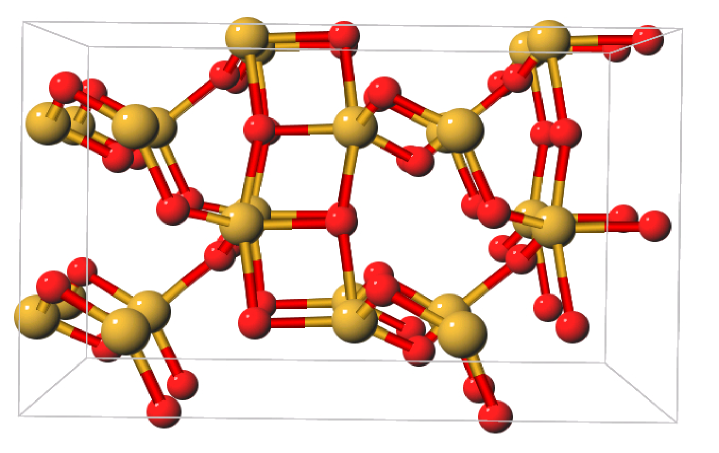
Figure 2: The optimal structure of quartz at the $\Gamma$-point RPBE/STO-3G level of theory. Note that the picture contains 8 neighboring unit cells for a better representation of intercell bonds.

Table 1: Optimization results for crystal structures at the PBE/STO-3G level of theory and in the $\Gamma$-point approximation, using the QUICCA algorithm.

	Number of	Optimum energy
Molecule	optimization steps	(a.u.)
polyethylene	8	-77.56774
boron-nitride	5	-78.41368
(10-0)carbon-nanotube	7	-1503.75024
ice	15	-301.31784
quartz	44	-1303.03159
sulfur	89	-12595.53586

We have developed a periodic test suite in the spirit of Baker’s gas phase set Baker (1993). The periodic test set includes 6 different systems: Polyethylene, hexagonal boron-nitride, a (10,0)carbon-nanotube, hexagonal ice Goto et al. (1990), quartz Tucker et al. (2001) and sulfur Gallacher and Pinkerton (1992). Most of these structures were taken either from the Inorganic Crystal Structures Database (ICSD) ICS (2004) or from Cambridge Crystallographic Data Center CCD (2004) and the translationally unique positions generated with Mercury Mer (2004). Details of the geometries used are given in Appendix A.

Full, simultaneous relaxation of both the lattice and atomic positions have been carried out by means of crystal QUICCA, described above, in the $\Gamma$-point approximation at the RPBE/STO-3G level of theory.

Table 1 shows the number of optimization steps and the optimal energy for each system. While the first four test systems converged quickly, quartz and sulfur took substantially longer to reach the optimum. In the case of quartz, there is a very large (unphysical) deformation, wherein four membered rings are formed during optimization, due perhaps to a combination of a minimal basis and $\Gamma$-point effects. The optimized structure of quartz is shown in Fig. 2. In the sulfur crystal, $S_{8}$ rings interact via a Van der Waals like interaction, which has a very flat potential, making this a challenging test case.

IV.1.1 Convergence of the energies

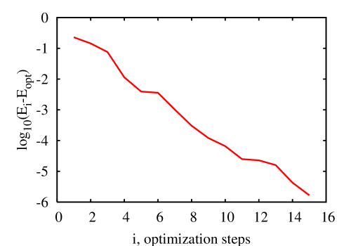
Figure 3: Convergence of the energy during the optimization of hexagonal ice.

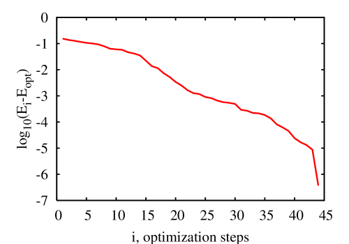
Figure 4: Convergence of the energy during the optimization of quartz.

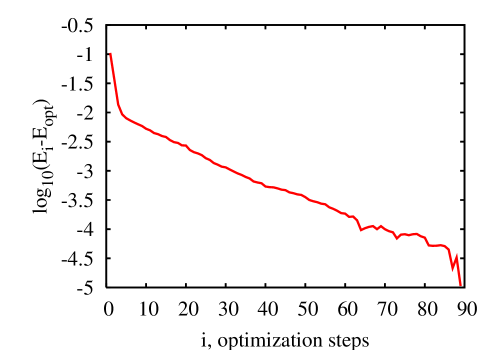
Figure 5: Convergence of the energy during the optimization of sulfur.

Convergence of the total energy is shown in Figs. 3-5 for ice, quartz and sulfur.

IV.1.2 Convergence of the gradients

Figures 6-8 show convergence of the maximum Cartesian gradients on atoms and lattice-vector gradients, $g_{{\rm max},i}$, with optimization step $i$.

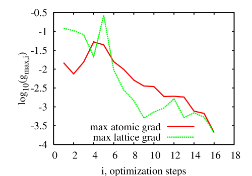
Figure 6: Convergence of the gradients during the optimization of hexagonal ice.

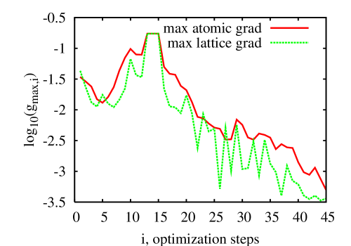
Figure 7: Convergence of the gradients during the optimization of quartz.

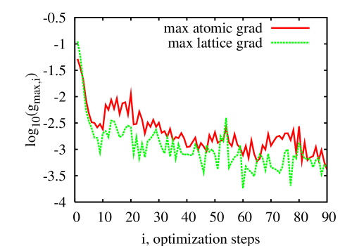
Figure 8: Convergence of the gradients during the optimization of sulfur.

IV.2 Urea

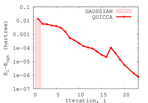
Figure 9: Convergence of the energy during full relaxation of RPBE/3-21G urea. The bar gives the energy difference computed by Kudin, Scuseria and Schlegel Kudin et al. (2001).

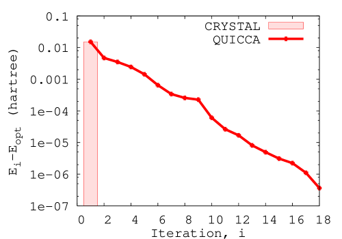
Figure 10: Convergence of the energy during lattice constrained optimization of RHF-MIC/STO-3G urea. The bar gives the energy difference given by Civalleri et. al Civalleri et al. (2001).

The experimental structure of urea, solved by Swaminanthan et. al Swaminathan et al. (1984), has been used as a benchmark for crystal optimization by several groups. Kudin, Scuseria and Schlegel Kudin et al. (2001) implemented an early internal coordinate optimization scheme in the GAUSSIAN programs, and applied it to the optimization of RPBE/3-21G urea with internal coordinate constraints. At about the same time, Civalleri et. al Civalleri et al. (2001) implemented a Cartesian conjugate gradient scheme in the CRYSTAL program, and carried out careful studies examining the effects of k-space sampling and integral tolerances on fixed lattice optimization of RHF/STO-3G urea.

Here, we make direct contact with these works, Refs.[Kudin et al., 2001; Civalleri et al., 2001]. However, because the linear scaling methods used by MondoSCF are $\Gamma$-point only, we employ a $2\times 2\times 2$ supercell, so that we may make approximate numerical comparison with the k-space methods. This $2\times 2\times 2$ supercell involves 16 urea molecules, $C_{1}$ (no) symmetry, 128 atoms in total, and more than 850 redundant internal coordinates; the number of internal coordinates used by QUICCA fluctuates slightly during optimization. For comparison, the work of Civalleri et. al Civalleri et al. (2001) makes use of $P\bar{4}2_{1}m$ symmetry, involving just 8 variables in the fixed lattice optimization of urea. In their relaxation of urea, Kudin, Scuseria and Schlegel Kudin et al. (2001) employed a 4 molecule cell with $S_{4}$ symmetry, with optimization of the lattice and atomic centers, but all dihedral angles constrained, involving 204 redundant internal coordinates.

Convergence of the RPBE/3-21G MondoSCF calculations are shown in Fig. 9, in which a full relaxation of lattice and atomic centers has been performed, together with the energy difference from Ref. [Kudin et al., 2001]. The GAUSSIAN values for this calculation, involving constrained dihedrals, are -447.6501595 and -447.6632120 for the beginning and ending values of the total energy. These (and subsequent) values have been normalized to total energy per 2 urea molecules. The corresponding MondoSCF values are -447.648312 and -447.661578. The GAUSSIAN energy difference is -0.01305, while the MondoSCF difference is -0.01326. The GAUSSIAN optimization converged in 13 steps, while QUICCA took 24 steps.

Convergence of the RHF-MIC/STO-3G MondoSCF calculations are shown in Fig. 10, together with the energy difference from Ref. [Civalleri et al., 2001], both corresponding to relaxation of atomic centers only. The beginning and ending CYRSTAL values for this calculation are -442.069368 and -442.084595, respectively. For MondoSCF, they are -442.069473 and -442.084671. The energy differences are -.01523 and -.01520 for CRYSTAL and MondoSCF, respectively. The CRYSTAL optimization converged in 15 steps, while QUICCA took 19 steps.

V Discussion

Overall, the behavior of QUICCA for crystal systems is similar to that of gas phase systems. For a well behaved system like ice, convergence is rapid and monotone. For systems undergoing large rearrangements, such as the quartz system, QUICCA takes many more steps, but still maintains monotone convergence. For both illconditioned (floppy) gas phase and crystal systems, such as sulfur, convergence is slower, with steps that sometimes raise the energy, even with 3-step backtracking.

Large amplitude motions can lead to rapid changes in curvature of the potential energy surface. In this case, the QUICCA algorithm may offer advantages relative to strategies based on BFGS-like updates, which are history laden. This is because QUICCA employs a weighting scheme that takes large moves into account and that can identify recently introduced trends in just a few steps.

The problems encountered with floppy systems are by no means unique to QUICCA, but plague most gradient only internal coordinate schemes. Also, as with other schemes, we have found the performance of QUICCA to be sensitive to the quality of the internal coordinate system. It is our opinion that the difficulties encountered with many floppy systems could be overcome with a better choice of internal coordinate system.

For floppy systems, the ability to resolve small energy differences with limited precision (due to linear scaling algorithms) can also be problematic. In particular, with the TIGHT option, MondoSCF tries to deliver a relative precision of 8 digits in the total energy, and 4 digits of absolute precision in forces. For sulfur, achieving atomic forces below 5D-4 corresponds to an energy difference of 1D-5, demanding a relative precision in the total energy of 1D-10. Exceeding the limits of the TIGHT energy threshold can be seen clearly in Fig. 5, wherein the energy has jumps below 1D-4. The observant reader will also notice that the $21^{\rm st}$ data point is missing from Fig. 9. This data point was removed because it was 1D-4 below the converged value of the total energy, -3581.2926, confusing the log-linear plot. These fluctuations are at the targeted energy resolution, and are likely due to changes in the adaptive HiCu grid for numerical integration of the exchange-correlation Tymczak et al. (2005). Nevertheless, reliable structural information can still be obtained, as absolute precision in the forces is retained with increasing system size, allowing gradient following algorithms such as QUICCA to still find a geometry which satisfies the force convergence criteria.

For the urea calculations, very good agreement was found between the MondoSCF calculations and the CRYSTAL results, in accordance with our previous experience for both pure DFT Tymczak et al. (2005) and RHF-MIC models Tymczak and Challacombe (2005). Slightly less satisfactory agreement was found between the MondoSCF and GAUSSIAN calculations, which was probably due to the differences in constraint. In both cases, the QUICCA calculations took more steps; 4 more than CRYSTAL, and 11 more than GAUSSIAN. It should be pointed out though, that the MondoSCF calculations involved a substantially more complicated potential energy surface: Firstly, the $\Gamma$-point surface lacks the symmetry provided by k-space sampling. Secondly, the $2\times 2\times 2$ calculation has many more degrees of freedom, and in particular, lower frequency modes due to the larger cell.

VI Conclusions

We have implemented the Bučko, Hafner and Ángyán Bučko et al. (2005) definition of periodic internal coordinates in conjunction with the QUICCA algorithm, and demonstrated efficient, full relaxation of systems with one, two and three dimensional periodicity. In general, we have found that QUICCA performs with an efficiency comparable to that of similarly posed gas phase problems, and speculate that further enhancement may be achieved through an improved choice of internal coordinates.

We have argued that linear scaling internal coordinate transformations for crystal systems can be achieved with a left-handed pseudo-inverse, as the dense rows and columns of the periodic ${\bf B}^{t}{\bf B}$ matrix determine just the last few pivots of the corresponding Cholesky factor.

We have carried out supercell calculations using a full compliment of linear scaling algorithms, including sparse linear algebra, fast force and matrix builds and found good agreement with k-space methods, involving a modest number of optimization cycles. Thus, in addition to further demonstrating the stability of our linear scaling algorithms, we have established QUICCA as a reliable tool for large scale optimization problems in the condensed phase.

In conclusion, QUICCA is a new gradient only approach to internal coordinate optimization that is robust and generally applicable, both to gas-phase molecules and systems of one, two and three dimensional periodicity. It allows for flexible optimization protocols, involving simultaneous relaxation of lattice and atom centers, constrained lattice with relaxation of atom centers, constrained atom centers with optimization of the lattice, admixtures of the above with constrained internal coordinates, etc. QUICCA is conceptually simple and easy to implement. Perhaps most importantly though, it is a new approach to gradient only internal coordinate optimization, offering a number of opportunities for further development.

Appendix A TEST SET COORDINATES

Here, input geometries for the crystal optimization test suite are detailed. These geometries are available as supplementary data, and are also available from the authors upon request.

Polyethylene

The 1-D periodic structure of polyethylene is given in Table 2.

Table 2: Atomic coordinates in $\AA$ for the elementary unit cell of polyethylene, with corresponding lattice parameters $a=2.0\AA,b=c=0.00,\alpha=\beta=\gamma=90.0^{\circ}$.

C	0.500	0.500	0.000
H	0.500	1.300	0.800
H	0.500	1.300	-0.800
C	1.500	-0.500	0.000
H	1.500	-1.300	0.800
H	1.500	-1.300	-0.800

Hexagonal boron-nitride

The 2-D periodic coordinates for hexagonal boron-nitride are given in Table 3.

Table 3: Fractional coordinates for the elementary unit cell of hexagonal boron-nitride with corresponding lattice parameters $a=b=2.420\AA,c=0.00,\alpha=\beta=90.0^{\circ},$ and $\gamma=120.0^{\circ}$.

B	0.33333333333	0.1666666666	0.00
N	0.66666666666	0.8400000000	0.00

(10,0)carbon-nanotube

The geometry of the 1-D periodic (10,0)carbon-nanotube has all bond-lengths parallel to the nanotube axis initially at $1.480$Å, while those running perpendicular to the axis are $1.402$Å long. The lattice length is $a=4.44$Å, with the elementary cell containing 40 atoms. While this data entirely determines the structure of the symmetric (10,0)carbon-nanotube, it is also available as supplementary data.

Ice

Hexagonal ice is the most important natural occurrence of ice. Its structure has been taken from the literature Goto et al. (1990). Since the literature provides two equilibrium position for each hydrogen atom, due to the tunneling of hydrogens in ice, our starting structure is taken as the average of these two positions for each hydrogen atom, and is given in Table 4.

Table 4: Atomic coordinates in $\AA$ for the elementary unit cell of hexagonal ice, with corresponding lattice parameters $a=b=4.511\AA,c=7.346\AA,\alpha=90.0^{\circ},\beta=90.0^{\circ}$ and $\gamma=120.0^{\circ}$

O	0.0000	2.6040000	3.216
H	2.2555	0.0003594	3.673
H	1.1280	1.9540000	3.673
O	2.2560	1.3020000	4.130
H	-1.1280	1.9540000	3.673
H	2.2560	1.3020000	5.510
O	2.2560	1.3020000	6.889
H	1.1280	1.9540000	7.346
H	-1.1280	1.9540000	7.346
O	0.0000	2.6040000	7.803
H	0.0000	2.6040000	9.183
H	2.2555	0.0003594	7.346

Quartz

The initial structure of quartz was taken from Ref. [Tucker et al., 2001], and has 9 atoms in the unit cell.

Table 5: Atomic coordinates in $\AA$ for the elementary unit cell of quartz, with corresponding lattice parameters $a=b=4.9019{\AA},c=5.3988{\AA},\alpha=\beta=90.0^{\circ}$ and $\gamma=120.0^{\circ}$.

Si	1.306	2.261	0.000
O	2.768	2.492	4.772
Si	-1.145	1.984	3.599
O	1.360	1.151	1.172
O	3.225	0.602	2.972
O	0.317	1.753	4.226
Si	2.291	0.000	1.800
O	-1.091	3.094	2.427
O	0.774	3.643	0.627

Sulfur

The structure of sulfur was taken from Ref. [Gallacher and Pinkerton, 1992]. Containing 32 atoms, this structure is available as supplementary data.