Multichannel quantum-defect theory for slow atomic collisions

Abstract

We present a multichannel quantum-defect theory for slow atomic collisions that takes advantages of the analytic solutions for the long-range potential, and both the energy and the angular-momentum insensitivities of the short-range parameters. The theory provides an accurate and complete account of scattering processes, including shape and Feshbach resonances, in terms of a few parameters such as the singlet and the triplet scattering lengths. As an example, results for ²³Na-²³Na scattering are presented and compared close-coupling calculations.

I Introduction

Slow atomic collisions are at the very foundation of cold-atom physics, since they determine how atoms interact with each other and how this interaction might be manipulated Stwalley (1976); Tiesinga et al. (1993). While substantial progress has been made over the past decade Weiner et al. (1999), there are still areas where the existing theoretical framework is less than optimal. For example, all existing numerical methods may have difficulty with numerical stability in treating ultracold collisions in partial waves other than the $s$ wave, because the classically forbidden region grows infinitely wide as one approaches the threshold. This difficulty becomes a serious issue when there is a shape resonance right at or very close to the threshold, as the usual argument that the $s$ wave scattering dominates would no longer be applicable. Another area where a more optimal formulation is desirable is analytic representation. Since much of our interest in cold atoms is in complex three-body and many-body physics, a simple, preferably analytical representation of cold collisions would not only be very helpful to experimentalists, but also make it much easier to incorporate accurate two-body physics in theories for three and many-atom systems. Existing formulations of cold collisions provide little analytical results especially in cases, such as the alkali-metal atoms, where the atomic interaction is complicated by hyperfine structures. Furthermore, whatever analytic results that we do have have been based almost exclusively on the effective-range theory Blatt and Jackson (1949), the applicability of which is severely limited by the long-range atomic interaction Gao (1998a, 2004a).

Built upon existing multichannel quantum-defect theories that are based either on free-particle reference functions or on numerical solutions for the long-range potential Mies (1980); Julienne and Mies (1989); Gao (1996); Burke, Jr. et al. (1998); Mies and Raoult (2000); Raoult and Mies (2004), we present here a multichannel, angular-momentum-insensitive, quantum-defect theory (MAQDT) that overcomes many of the limitations of existing formulations. It is a generalization of its single-channel counterpart Gao (2001, 2000, 2004b), and takes full advantage of both the analytic solutions for the long-range potential Gao (1998b, 1999), and the angular momentum insensitivity of a properly defined short-range K matrix $K^{c}$ Gao (2001, 2004b). We show that as far as $K^{c}$ is concerned, the hyperfine interaction can be ignored, and the frame transformation Rau and Fano (1971); Lee and Lu (1973); Lee (1975); Gao (1996); Burke, Jr. et al. (1998) applies basically exactly. This conclusion greatly simplifies the description of any atomic collision that involves hyperfine structures. In the case of a collision between any two alkali-metal atoms in their ground state, whether they are identical or not, it reduces a complex multichannel problem to two single channel problems. This property, along with the energy and angular-momentum insensitivity of $K^{c}$ Gao (2001, 2004b), leads to an accurate and complete characterization of slow collisions between any two alkali-metal atoms, including shape resonances, Feshbach resonances, practically all partial waves of interest, and over an energy-range of hundreds of millikelvins, by four parameters for atoms with identical nuclei, and five parameters for different atoms or different isotopes of the same atom. To be more specific, the four parameters can be taken as the singlet $s$ wave scattering length $a_{0S}$, the triplet $s$ wave scattering length $a_{0T}$, the $C_{6}$ coefficient for the long-range van der Waals potential $-C_{6}/r^{6}$, and the atomic hyperfine splitting $\Delta E^{HF}_{a}$ (The reduced mass $\mu$, which is also needed, is not counted as a parameter since it is always fixed and well-known). For different atoms or different isotopes of the same atom, we need another hyperfine splitting for a total of five parameters. These results also prepare us for future analytic representations of multichannel cold collisions, when we restrict ourselves to a smaller range of energies.

II MAQDT

An $N$-channel, two-body problem can generally be described by a set of wave functions

$$\psi_{j}=\sum_{i=1}^{N}\Phi_{i}F_{ij}(r)/r\;,$$ (1)

Here $\Phi_{i}$ are the channel functions describing all degrees of freedom other than the inter-particle distance $r$; and $F_{ij}(r)$ satisfies a set of close-coupling equations

$$\left[-\frac{\hbar^{2}}{2\mu}\frac{d^{2}}{dr^{2}}+\frac{\hbar^{2}l_{i}(l_{i}+1)}{2\mu r^{2}}-E\right]F_{ij}+\sum_{j=1}^{N}V_{ij}(r)F_{ij}=0\;,$$ (2)

where $\mu$ is the reduced mass; $l_{i}$ is the relative angular momentum in channel $i$; $E$ is the total energy; and $V_{ij}$ is the representation of inter-particle potential in the set of chosen channels (see, e.g., reference Gao (1996) for a diatomic system with hyperfine structures).

Consider now a class of problems for which the potential at large distances ($r\geq r_{0}$) is of the form of

$$V_{ij}(r)=(E_{i}-C_{n_{i}}/r^{n_{i}})\delta_{ij}\;,$$ (3)

in the fragmentation channels that diagonalize the long-range interactions. Here $n_{i}>2$, and $E_{i}$ is the threshold energy associated with a fragmentation channel $i$. As an example, for the scattering of two alkali-metal atoms in their ground state, the fragmentation channels in the absence of any external magnetic field are characterized by the $FF$ coupling of reference Gao (1996); differences in threshold energies originate from atom hyperfine interaction; $n_{i}=6$ corresponds to the van der Waals interaction; and $r_{0}$, with an order of magnitude around 30 a.u., corresponds to the range of exchange interaction.

Before enforcing the physical boundary condition (namely the condition that a wave function has to be finite everywhere) at infinity, Eqs. (2) have $N$ linearly independent solutions that satisfy the boundary conditions at the origin. For $r\geq r_{0}$, one set of these solutions can be written as

$$\psi^{c}_{j}=\sum_{i=1}^{N}\Phi_{i}(f^{c}_{i}\delta_{ij}-g^{c}_{i}K^{c}_{ij})/r\;.$$ (4)

Here $f^{c}_{i}$ and $g^{c}_{i}$ are the reference functions for the long-range potential, $-C_{n_{i}}/r^{n_{i}}$, in channel $i$, at energy $\epsilon_{i}=E-E_{i}$. They are chosen such that they are independent of both the channel kinetic energy $\epsilon_{i}$ and the relative angular momentum $l_{i}$ at distances much smaller than the length scale $\beta_{n_{i}}=(2\mu C_{n_{i}}/\hbar^{2})^{1/(n_{i}-2)}$ associated with the long-range interaction (see Appendix A and references Gao (2001, 2004b)).

Equation (4) defines the short-range K matrix $K^{c}$. It has a dimension equal to the total number of channels, $N$, and encapsulates all the short-range physics. The $K^{c}$ matrix can either be obtained from numerical calculations (see Appendix B) or be inferred from other physical quantities such as the singlet and the triplet scattering lengths, as discussed later in the article.

At energies where all $N$ channels are open, the solutions given by Eq. (4) already satisfy the physical boundary conditions at infinity. Using the asymptotic behaviors of reference functions $f^{c}$ and $g^{c}$ at large $r$ (see Appendix A and reference Gao (1998b)), it is easy to show from Eq. (4) that the physical $K$ matrix, defined by Eqs. (4) and (5) of reference Gao (1996), is an $N\times N$ matrix given in terms of $K^{c}$ by

$$K(E)=-(Z^{c}_{fg}-Z^{c}_{gg}K^{c})(Z^{c}_{ff}-Z^{c}_{gf}K^{c})^{-1}\;.$$ (5)

Here $Z^{c}_{fg},Z^{c}_{gg},Z^{c}_{ff}$, and $Z^{c}_{gf}$ are $N\times N$ diagonal matrices with diagonal elements given by $Z^{c(n_{i})}_{fg}(\epsilon_{i},l_{i}),Z^{c(n_{i})}_{gg}(\epsilon_{i},l_{i}),Z^{c(n_{i})}_{ff}(\epsilon_{i},l_{i})$, and $Z^{c(n_{i})}_{gf}(\epsilon_{i},l_{i})$, respectively (see Appendix A and references Gao (1998b, 2000)). Equation (5) is of the same form as its single channel counterpart Gao (2001, 2000), except that the relevant quantities are now matrices, and $K^{c}$ is generally not diagonal.

At energies where $N_{o}$ of the channels are open ($\epsilon_{i}>0$, for $i\in o$), and $N_{c}=N-N_{o}$ of the channels are closed ($\epsilon_{i}<0$, for $i\in c$), the physical boundary conditions at infinity leads to $N_{c}$ conditions that reduce that number of linearly independent solutions to $N_{o}$ Seaton (1983); Gao (1996); Burke, Jr. et al. (1998). The asymptotic behavior of these $N_{o}$ solutions gives the $N_{o}\times N_{o}$ physical $K$ matrix

$$K(E)=-(Z^{c}_{fg}-Z^{c}_{gg}K^{c}_{eff})(Z^{c}_{ff}-Z^{c}_{gf}K^{c}_{eff})^{-1}\;.$$ (6)

Here $Z^{c}_{fg},Z^{c}_{gg},Z^{c}_{ff}$, and $Z^{c}_{gf}$ are $N_{o}\times N_{o}$ diagonal matrices with diagonal elements given by the corresponding $Z^{c}$ matrix element for all open channels; and we have defined the effective $K^{c}$ matrix for the open channels, $K^{c}_{eff}$, to be

$$K^{c}_{eff}=K^{c}_{oo}+K^{c}_{oc}(\chi^{c}-K^{c}_{cc})^{-1}K^{c}_{co}\;.$$ (7)

Here $\chi^{c}$ is an $N_{c}\times N_{c}$ diagonal matrix with elements $\chi^{c(n_{i})}(\epsilon_{i},l_{i})$ (see Appendix A and references Gao (1998b, 2001)) for all closed channels. $K^{c}_{oo}$, $K^{c}_{oc}$, $K^{c}_{co}$, $K^{c}_{cc}$, are submatrices of $K^{c}$ corresponding to open-open, open-closed, closed-open, and closed-closed channels, respectively.

All on-the-energy-shell scattering properties can be derived from the physical $K$ matrix. In particular, the physical $S$ matrix is given by Gao (1996)

$$S(E)=[I+iK(E)][I-iK(E)]^{-1}\;,$$ (8)

where $I$ represents a unit matrix. From the $S$ matrix, the scattering amplitudes, the differential cross sections, and other physical observables associated with scattering can be easily deduced Gao (1996).

It is worth noting that Eq. (6) preserve the form of Eq. (5). Thus the effect of closed channels is simply to introduce an energy dependence, through $\chi^{c}$, into the effective $K^{c}$ matrix, $K^{c}_{eff}$, for the open channels. In particular, the bare (unshifted) locations of Feshbach resonances, if there are any, are determined by the solutions of

$$\det[\chi^{c}(E)-K^{c}_{cc}]=0\;.$$ (9)

They are locations of would-be bound states if the closed channels are not coupled to the open channels. The same equation also gives the bound spectrum of true bound states, at energies where all channels are closed.

This completes our summary of MAQDT. It is completely rigorous with no approximations involved. The theory is easily incorporated into any numerical calculations (see Appendix B). The difference from the standard approach is that one matches the numerical wave function to the solutions of the long-range potential to extract $K^{c}$, instead of matching to the free-particle solutions to extract $K$ directly. This procedure converges at a much smaller $r=r_{0}$, the range of the exchange interaction, than methods that match to the free-particle solutions. Furthermore, since the propagation of the wave function from $r_{0}$ to infinity is done analytically, through the $Z^{c}$ matrix for open channels and $\chi^{c}$ function for closed channels, there is no difficulty in treating shape resonances right at or very close to the threshold. This improved convergence and stability does not however fully illustrate the power of MAQDT formulation and is not the focus of this article. Instead, we focus here on the simple parameterization of slow atomic collisions with hyperfine structures made possible by MAQDT. The result also lays the ground work for future analytic representations of cold collisions.

III Simplified parameterization with frame transformation

Equations (5)-(7), and (9) already provide a parameterization of slow-atom collisions and diatomic bound spectra in terms of the elements of the $K^{c}$ matrix. For alkali-metal atoms in their ground state, where the multichannel nature arises from the hyperfine interaction, or a combination of hyperfine and Zeeman interactions for scattering in a magnetic field, this parameterization can be simplified much further by taking advantage of a frame transformation Rau and Fano (1971); Lee and Lu (1973); Lee (1975); Gao (1996); Burke, Jr. et al. (1998).

At energies comparable to, or smaller than the atomic hyperfine and/or Zeeman splitting, one faces the dichotomy that the hyperfine and/or Zeeman interaction, while weak compared to the typical atomic interaction energy, is sufficiently strong that the physical K matrix changes significantly over a hyperfine splitting. (This is reflected in the very existence of Feshbach resonances Stwalley (1976); Tiesinga et al. (1993) and states with binding energies comparable to or small than the hyperfine splitting.) As a result, the frame transformation does not apply directly to the physical K matrix itself, and is generally a bad approximation even for the $K^{0}$ matrix of reference Gao (1996). It was this recognition that first motivated the solutions for the long-range potentials Gao (1998b, 1999).

This dichotomy is easily and automatically resolved with the introduction of the short range K matrix $K^{c}$. The solution is simply to ignore the hyperfine and/or Zeeman interaction only at small distances and treat it exactly at large distances. For $r<r_{0}$, the atomic interaction is of the order of the typical electronic energy. Thus as far as $K^{c}$, which converges at $r_{0}$, is concerned, the hyperfine and/or Zeeman interaction can be safely ignored. In this approximation, the $K^{c}$ matrix in the fragmentation channels can be obtained from the $K^{c}$ matrix in the condensation channels, namely the channels that diagonalize the short-range interactions, by a frame transformation.

For simplicity, we restrict ourselves here to the case of zero external magnetic field, although the theory can readily be generalized to include a magnetic field. The fragmentation channels are the $FF$ coupled channels characterized by quantum numbers Gao (1996):

$$(\alpha_{1}L_{1}S_{1}J_{1}I_{1}F_{1})_{A}(\alpha_{2}L_{2}S_{2}J_{2}I_{2}F_{2})_{B}FlTM_{T}\;,$$

where $F$ results from the coupling of $F_{1}$ and $F_{2}$; $l$ is the relative orbital angular momentum of the center-of-masses of the two atoms. $T$ represents the total angular momentum, and $M_{T}$ is its projection on a space-fixed axis Gao (1996).

Provided that the off-diagonal second-order spin-orbital coupling Mies et al. (1996) can be ignored, a good approximation for lighter alkali-metal atoms, or more generally, for any physical processes that are allowed by the exchange interaction, the condensation channels can be taken as the $LS$ coupled channels characterized by quantum numbers Gao (1996):

$$(\alpha_{1}L_{1}S_{1}I_{1})_{A}(\alpha_{2}L_{2}S_{2}I_{2})_{B}Ll{\cal L}SKITM_{T}\;,$$

where $\mathbf{\cal L}=\mathbf{L}+\mathbf{l}$ is the total orbital angular momentum. $\mathbf{S}=\mathbf{S}_{1}+\mathbf{S}_{2}$ is the total electron spin. $\mathbf{I}=\mathbf{I}_{1}+\mathbf{I}_{2}$ is the total nuclear spin. And $\mathbf{K}=\mathbf{\cal L}+\mathbf{S}$ is the total angular momentum excluding nuclear spin.

Ignoring hyperfine interactions, as argued earlier, the $K^{c}$ matrix in $FF$-coupled channels, labeled by index $i$ or $j$, is related to the $K^{c}$ matrix in $LS$-coupled channels, labeled by index $\alpha$ or $\beta$, by a frame transformation Gao (1996)

$$K^{c}_{ij}=\sum_{\alpha\beta}U_{i\alpha}K^{c(LS)}_{\alpha\beta}U_{j\beta}\;,$$ (10)

where $K^{c(LS)}$ is the $K^{c}$ matrix computed in the LS coupling with the hyperfine interactions ignored. The most general form of frame transformation $U_{j\beta}$ is given by Eq. (49) of reference Gao (1996). For collision between any two atoms with zero orbital angular momentum, $L_{1}=L_{2}=L=0$, including of course any two alkali-metal atoms in their ground states, the frame transformation simplifies to

$$U_{i\beta}(T) = \delta_{l_{i}l_{\beta}}(-1)^{F_{i}+S_{\beta}+I_{\beta}}[F_{1i},F_{2i},F_{i},S_{\beta},K_{\beta},I_{\beta}]^{1/2}$$ (16)

$$\times\left\{\begin{array}[]{ccc}F_{i}&l_{i}&T\\ K_{\beta}&I_{\beta}&S_{\beta}\end{array}\right\}\left\{\begin{array}[]{ccc}S_{1}&S_{2}&S_{\beta}\\ I_{1}&I_{2}&I_{\beta}\\ F_{1i}&F_{2i}&F_{i}\end{array}\right\}\;,$$

for atoms with different nuclei. Here $[a,b,\dots]\equiv(2a+1)(2b+1)\cdots$. For two atoms with identical nuclei, the same transformation needs to be multiplied by a normalization factor Gao (1996)

$$U_{\{i\}\{\beta\}} = \{1+\delta(\alpha_{2}L_{2}S_{2},\alpha_{1}L_{1}S_{1})[1-\delta(J_{2i}F_{2i},J_{1i}F_{1i})]\}^{1/2}$$ (17)

$$\times U_{i\beta}\;.$$

We emphasize that to the degree that the hyperfine interaction in a slow atomic collision can be approximated by atomic hyperfine interactions, as has always been assumed Tiesinga et al. (1993), the frame transformation given by Eq. (10) should be regarded as exact. If the hyperfine interaction inside $r_{0}$, the range of the exchange interaction, cannot be ignored, the true molecular hyperfine interaction Babb and Dalgarno (1991) would have to be used. Inclusion of atomic hyperfine interactions inside $r_{0}$ is simply another approximation, and an unnecessary complication, that is of the same order of accuracy as ignoring it completely. In other words, any real improvement over the frame transformation has to require a better treatment of molecular hyperfine interactions Babb and Dalgarno (1991). A similar statement is also applicable to the Zeeman interaction.

The applicability of the frame transformation greatly simplifies the description of any slow atomic collision with hyperfine structures. For alkali-metal atoms in their ground state, and ignoring off-diagonal second-order spin-orbital coupling Mies et al. (1996), it reduces a complex multichannel problem to two single channel problems, one for the singlet $S=0$, and one for the triplet, $S=1$, with their respective single-channel $K^{c}$ Gao (2001, 2000) denoted by $K^{c}_{S}(\epsilon,l_{i})$ and $K^{c}_{T}(\epsilon,l_{i})$, respectively. The $K^{c}$ matrix in the LS coupling, $K^{c(LS)}$, is diagonal with diagonal elements given by either $K^{c}_{S}$ or $K^{c}_{T}$ Gao (1996). Ignoring the energy and the angular momentum dependences of $K^{c}_{S}(\epsilon,l_{i})$ and $K^{c}_{T}(\epsilon,l_{i})$ Gao (2001, 2004b), they become simply two parameters $K^{c}_{S}=K^{c}_{S}(0,0)$ and $K^{c}_{T}=K^{c}_{T}(0,0)$, which are related to the singlet and the triplet $s$ wave scattering lengths by Gao (2003)

$$a_{0}/\beta_{n}=\left[b^{2b}\frac{\Gamma(1-b)}{\Gamma(1+b)}\right]\frac{K^{c}(0,0)+\tan(\pi b/2)}{K^{c}(0,0)-\tan(\pi b/2)}\;,$$ (18)

where $b=1/(n-2)$ with $n=6$ for alkali-metal scattering in the ground state. With $K^{c(LS)}$, and therefore $K^{c}$, being parameterized by two parameters, a complete parameterization of alkali-metal scattering requires only two, or three, more parameters including $C_{6}$, which determined the length and energy scales for the long range interaction, and the atomic hyperfine splitting $\Delta E^{HF}_{a}$, which characterizes the strength of atomic hyperfine interaction and also determines the channel energies.

We note here that our formulation ignores the weak magnetic dipole-dipole interaction Stoof et al. (1988); Mies et al. (1996). It is important only for processes, such as the dipolar relaxation, that are not allowed by the exchange interaction. Such processes can be incorporated perturbatively after a MAQDT treatment Mies and Raoult (2000). We also note that for processes, such as the spin relaxation of Cs, for which the off-diagonal second-order spin-orbital coupling is important Mies et al. (1996); Leo et al. (2000), a different choice of condensation channels, similar to the $JJ$-coupled channels of reference Gao (1996), would be required. The resulting description is similar conceptually, but involves more parameters Mies et al. (1996); Leo et al. (2000).

IV Sample results for sodium-sodium scattering

As an example, Figures 1-3 show the comparison between close-coupling calculations and a four-parameter MAQDT parameterization for slow atomic collision between a pair of ²³Na atoms in the absence of exteranl magnetic field. The points are the close-coupling results using the potentials of references Samuelis et al. (2000); Laue et al. (2002). The curves represent the results of a four-parameter parameterization with $a_{0S}=19.69$ a.u., $a_{0T}=64.57$ a.u., $C_{6}=1556$ a.u. Derevianko et al. (1999), and $\delta E^{HF}_{a}=1772$ MHz, where $a_{0S}$ and $a_{0T}$ are computed from the singlet and the triplet potentials of references Samuelis et al. (2000); Laue et al. (2002). Figure 1 shows the $S$ matrix element for the $s$ wave elastic scattering in channel [$\{F_{1}=1,F_{2}=1\}F=0,l=0,T=0$]. The feature around 130 mK is a Feshbach resonance in channel [$\{F_{1}=2,F_{2}=2\}F=0,l=0,T=0$].

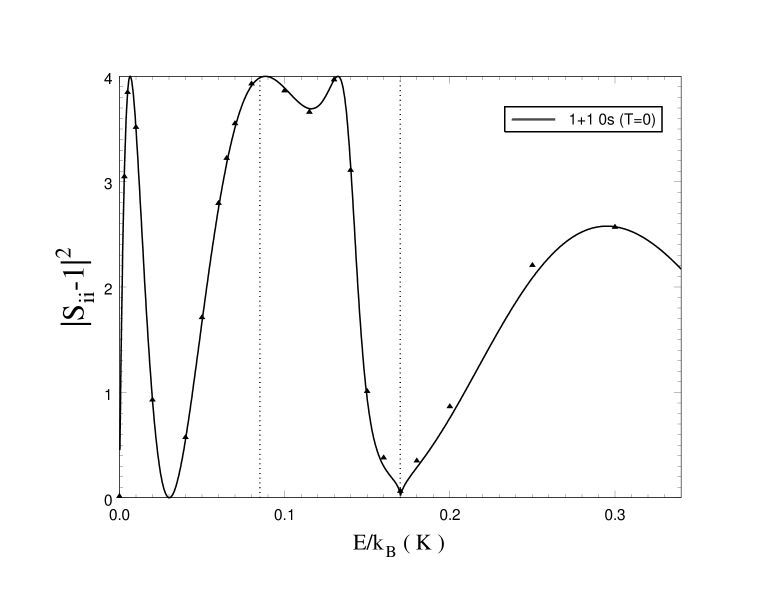
Figure 1: $|S_{ii}-1|^{2}$, where $S_{ii}$ is an $S$ matrix element, for the $s$ wave elastic scattering of two ²³Na atoms in channel [$\{F_{1}=1,F_{2}=1\}F=0,l=0,T=0$], as a function of $E/k_{B}$, where $k_{B}$ is the Boltzmann constant. The vertical lines identify the locations of thresholds for $\{F_{1}=1,F_{2}=2\}$ and $\{F_{1}=2,F_{2}=2\}$ channels. Solid line: results of a four-parameter MAQDT parameterization. Points: results of close-coupling calculations.

For this particular case, $K^{c(LS)}$ is a $2\times 2$ matrix

$$K^{c(LS)}=\left(\begin{array}[]{cc}K^{c}_{S}&0\\ 0&K^{c}_{T}\end{array}\right)\;,$$ (19)

with channel ordering shown in Table 1.

Table 1: Channel structure for $s$ wave scattering between two identical atoms with $L_{1}=L_{2}=0$, $S_{1}=S_{2}=1/2$, and $I_{1}=I_{2}=3/2$, in the absence of external magnetic field. Examples include ⁷Li, ²³Na, ³⁹K and ⁸⁷Rb.

$T$	LS coupling $(S,I)$	FF coupling $\{F_{1},F_{2}\}F$
0	S=0, I=0	{1,1}0
	S=1, I=1	{2,2}0
1	S=1, I=1	{1,2}1
2	S=0, I=2	{1,1}2
	S=1, I=1	{1,2}2
	S=1, I=3	{2,2}2
3	S=1, I=3	{1,2}3
4	S=1, I=3	{2,2}4

$K^{c}_{S}$ and $K^{c}_{T}$ are related to the singlet and the triplet scattering lengths by Eq. (18). The frame transformation is given by [c.f. Eqs. (16) and (17)]

$$U(T=0)=\frac{1}{2\sqrt{2}}\left(\begin{array}[]{cc}\sqrt{3}&\sqrt{5}\\ \sqrt{5}&-\sqrt{3}\end{array}\right)\;,$$ (20)

which leads to

$$K^{c}=\frac{1}{8}\left(\begin{array}[]{cc}3K^{c}_{S}+5K^{c}_{T}&\sqrt{15}\left(K^{c}_{S}-K^{c}_{T}\right)\\ \sqrt{15}\left(K^{c}_{S}-K^{c}_{T}\right)&5K^{c}_{S}+3K^{c}_{T}\end{array}\right)\;.$$ (21)

From the $K^{c}$ matrix, the $S$ matrix is obtained from the MAQDT equations (5)-(8). Note how Eq. (21) shows explicitly that the off-diagonal element of $K^{c}$, which determines the rate of inelastic collision due to exchange interaction, goes to zero for $K^{c}_{S}=K^{c}_{T}$, namely when $a_{0S}=a_{0T}$.

The results presented in Figs. 2 and 3 are obtained in similar fashion. Figure 2 shows the $S$ matrix element for the $d$ wave elastic scattering in channel [$\{F_{1}=1,F_{2}=1\}F=2,l=2,T=2$]. It illustrates how the same parameters that we use to describe the $s$ wave scattering also describe the $d$ wave scattering, due to the fact that $K^{c}_{S}$ and $K^{c}_{T}$ are insensitive to $l$ Gao (2001, 2004b). Here the sharp features around the thresholds are $d$ wave shape resonances.

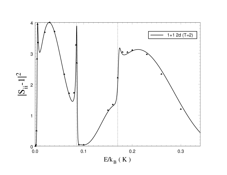
Figure 2: The same as Figure 1 excepts it is for $d$ wave channel [$\{F_{1}=1,F_{2}=1\}F=2,l=2,T=2$].

Figure 3 shows the $S$ matrix element for the $s$ wave inelastic scattering between channel [$\{F_{1}=1,F_{2}=1\}F=2,l=0,T=2$] and channel [$\{F_{1}=1,F_{2}=2\}F=2,l=0,T=2$].

Figure 3: The $S$ matrix element, $|S_{ij}|^{2}$, for the $s$ wave inelastic scattering of two ²³Na atoms between channels [$\{F_{1}=1,F_{2}=1\}F=2,l=0,T=2$] and [$\{F_{1}=1,F_{2}=2\}F=2,l=0,T=2$].

The kinks (discontinuities in the derivative), in both Fig. 3 and Fig. 1 at the $\{F_{1}=2,F_{2}=2\}$ threshold, are general features associated with the opening of an $s$ wave channel. There is no kink at the $\{F_{1}=1,F_{2}=2\}$ threshold in Figure 1 because the [$\{F_{1}=1,F_{2}=1\}F=0,l=0,T=0$] channel is not coupled to $\{F_{1}=1,F_{2}=2\}$ channels.

The agreements between the MAQDT parameterization and close-coupling calculations are excellent, exact for all practical purposes, in all cases. Conceptually, these results illustrate that through a proper MAQDT formulation, atomic collision over a wide range of energies (300 mK compared to the Doppler cooling limit of about 0.2 mK for ²³Na), with complex structures including Feshbach and shape resonances, and for different partial waves, can all be described by parameters that we often associate with the $s$ wave scattering at zero energy only, namely the singlet and the triplet scattering lengths.

V Conclusion

In conclusion, a multichannel, angular-momentum-insensitive, quantum-defect theory (MAQDT) for slow atomic collisions has been presented. We believe it to be the optimal formulation for purposes including exact numerical calculation, parameterization, and analytic representation. We have shown that by dealing with the short-range K matrix $K^{c}$, the frame transformation becomes basically exact, which greatly simplifies the description of any slow atomic collision with hyperfine structures. As an example, we have shown that even a simplest parameterization with four parameters, in which the energy and the $l$ dependence of $K^{c}_{S}$ and $K^{c}_{T}$ are completely ignored, reproduces the close-coupling calculations for ²³Na atoms over a wide range of energies basically exactly. The effect of an external magnetic field, which is not considered in this article, is easily incorporated as it simply requires another frame transformation Burke, Jr. et al. (1998).

The concepts and the main constructs of the theory can be generalized to other scattering processes including ion-atom scattering and atom-atom scattering in excited states. The key difference will be in the long-range interaction [c.f. Eq. (3)]. In addition to possibly different long-range exponent $n_{i}$ (such as $n_{i}=4$ for ion-atom scattering), there may also be long-range off-diagonal coupling that will have to be treated differently.

Finally, we expect that if we restrict ourselves to a smaller range of energies, of the order of $(\hbar^{2}/2\mu)(1/\beta_{6})^{2}$ (about 1 mK for ²³Na), a number of analytic results, similar to the single-channel results of references Gao (1998a) and Gao (2004a), can be derived even for the complex multichannel problem of alkali-metal collisions. These results may, in particular, lead to a more general and more rigorous parameterization of magnetic Feshbach resonances (see, e.g., references Marcelis et al. (2004); Raoult and Mies (2004) for some recent works in this area).

Appendix A Definitions of MAQDT functions

The reference functions $f^{c}$ and $g^{c}$ for a $-C_{n}/r^{n}$ ($n>2$) potential are a pair of linearly independent solutions of the radial Schrödinger equation

$$\left[-\frac{\hbar^{2}}{2\mu}\frac{d^{2}}{dr^{2}}+\frac{\hbar^{2}l(l+1)}{2\mu r^{2}}-\frac{C_{n}}{r^{n}}-\epsilon\right]u_{\epsilon l}(r)=0\;,$$ (22)

which can be written in a dimensionless form as

$$\left[\frac{d^{2}}{dr_{s}^{2}}-\frac{l(l+1)}{r_{s}^{2}}+\frac{1}{r_{s}^{n}}+\epsilon_{s}\right]u_{\epsilon_{s}l}(r_{s})=0\;,$$ (23)

where $r_{s}=r/\beta_{n}$ is a scaled radius, $\beta_{n}\equiv(2\mu C_{n}/\hbar^{2})^{1/(n-2)}$ is the length scale associated with the $-C_{n}/r^{n}$ interaction, and

$$\epsilon_{s}=\frac{\epsilon}{(\hbar^{2}/2\mu)(1/\beta_{n})^{2}}\;,$$ (24)

is a scaled energy.

The $f^{c}$ and $g^{c}$ pair are chosen such that they have not only energy-independent, but also angular-momentum-independent behaviors in the region of $r\ll\beta_{n}$ (namely $r_{s}\ll 1$):

$$f^{c}_{\epsilon_{s}l}(r_{s}) \stackrel{{\scriptstyle r_{s}\ll 1}}{{\longrightarrow}} (2/\pi)^{1/2}r_{s}^{n/4}\cos\left(y-\pi/4\right)\;,$$ (25)

$$g^{c}_{\epsilon_{s}l}(r_{s}) \stackrel{{\scriptstyle r_{s}\ll 1}}{{\longrightarrow}} -(2/\pi)^{1/2}r_{s}^{n/4}\sin\left(y-\pi/4\right)\;,$$ (26)

for all energies Gao (2001, 2003). Here $y=[2/(n-2)]r_{s}^{-(n-2)/2}$. They are normalized such that

$$W(f^{c},g^{c})\equiv f^{c}\frac{dg^{c}}{dr_{s}}-\frac{df^{c}}{dr_{s}}g^{c}=2/\pi\;.$$ (27)

For $\epsilon=0$, the $f^{c}$ and $g^{c}$ pair for arbitrary $n$ can be found in reference Gao (2004b). For $\epsilon\neq 0$, the $f^{c}$ and $g^{c}$ pair for $n=6$ can be found in reference Gao (2004c). The are related to the $f^{0}$ and $g^{0}$ pair of reference Gao (1998b) by

$$\left(\begin{array}[]{c}f^{c}\\ g^{c}\end{array}\right)=\frac{1}{\sqrt{2}}\left(\begin{array}[]{cc}\cos(\pi\nu_{0}/2)&\sin(\pi\nu_{0}/2)\\ -\sin(\pi\nu_{0}/2)&\cos(\pi\nu_{0}/2)\end{array}\right)\left(\begin{array}[]{cc}1&0\\ 0&-1\end{array}\right)\left(\begin{array}[]{c}f^{0}\\ g^{0}\end{array}\right)\;,$$ (28)

where $\nu_{0}=(2l+1)/4$ for $n=6$.

The $Z^{c(n)}(\epsilon_{s},l)$ matrix is defined by the large-$r$ asymptotic behaviors of $f^{c}$ and $g^{c}$ for $\epsilon>0$

$$f^{c}_{\epsilon_{s}l}(r_{s}) \stackrel{{\scriptstyle r\rightarrow\infty}}{{\longrightarrow}} \sqrt{\frac{2}{\pi k_{s}}}\left[Z^{c(n)}_{ff}(\epsilon_{s},l)\sin\left(k_{s}r_{s}-\frac{l\pi}{2}\right)-Z^{c(n)}_{fg}(\epsilon_{s},l)\cos\left(k_{s}r_{s}-\frac{l\pi}{2}\right)\right]\;,$$ (29)

$$g^{c}_{\epsilon_{s}l}(r_{s}) \stackrel{{\scriptstyle r\rightarrow\infty}}{{\longrightarrow}} \sqrt{\frac{2}{\pi k_{s}}}\left[Z^{c(n)}_{gf}(\epsilon_{s},l)\sin\left(k_{s}r_{s}-\frac{l\pi}{2}\right)-Z^{c(n)}_{gg}(\epsilon_{s},l)\cos\left(k_{s}r_{s}-\frac{l\pi}{2}\right)\right]\;,$$ (30)

where $k_{s}=k\beta_{n}$ with $k=(2\mu\epsilon/\hbar^{2})^{1/2}$. This define a $2\times 2$ $Z^{c(n)}(\epsilon_{s},l)$ matrix

$$Z^{c(n)}=\left(\begin{array}[]{cc}Z^{c(n)}_{ff}&Z^{c(n)}_{fg}\\ Z^{c(n)}_{gf}&Z^{c(n)}_{gg}\end{array}\right)\;.$$ (31)

It is normalized such that

$$\det\left[Z^{c(n)}\right]=Z^{c(n)}_{ff}Z^{c(n)}_{gg}-Z^{c(n)}_{gf}Z^{c(n)}_{fg}=1\;.$$ (32)

The $\chi^{c(n)}_{l}(\epsilon_{s})$ function is defined through the large-$r$ asymptotic behaviors of $f^{c}$ and $g^{c}$ for $\epsilon<0$.

$$f^{c}_{\epsilon_{s}l}(r_{s}) \stackrel{{\scriptstyle r\rightarrow\infty}}{{\longrightarrow}} (2\pi\kappa_{s})^{-1/2}\left[W^{c(n)}_{f-}(\epsilon_{s},l)e^{\kappa_{s}r_{s}}-W^{c(n)}_{f+}(\epsilon_{s},l)(2e^{-\kappa_{i}r})\right]\;,$$ (33)

$$g^{c}_{\epsilon_{s}l}(r_{s}) \stackrel{{\scriptstyle r\rightarrow\infty}}{{\longrightarrow}} (2\pi\kappa_{s})^{-1/2}\left[W^{c(n)}_{g-}(\epsilon_{s},l)e^{\kappa_{s}r_{s}}-W^{c(n)}_{g+}(\epsilon_{s},l)(2e^{-\kappa_{s}r_{s}})\right]\;,$$ (34)

where $\kappa_{s}=\kappa\beta_{n}$ with $\kappa=(2\mu|\epsilon_{i}|/\hbar^{2})^{1/2}$. This defines a $2\times 2$ $W^{c(n)}(\epsilon_{s},l)$ matrix,

$$W^{c(n)}=\left(\begin{array}[]{cc}W^{c(n)}_{f-}&W^{c(n)}_{f+}\\ W^{c(n)}_{g-}&W^{c(n)}_{g+}\end{array}\right)\;,$$ (35)

from which the $\chi^{c(n)}_{l}(\epsilon_{s})$ function is defined by

$$\chi^{c(n)}_{l}(\epsilon_{s})=W^{c(n)}_{f-}/W^{c(n)}_{g-}\;.$$ (36)

The $W^{c(n)}$ matrix is normalized such that

$$\det\left[W^{c(n)}\right]=W^{c(n)}_{f-}W^{c(n)}_{g+}-W^{c(n)}_{g-}W^{c(n)}_{f+}=1\;.$$ (37)

The $Z^{c(n)}(\epsilon_{s},l)$ and $W^{c(n)}(\epsilon_{s},l)$ matrices, for $\epsilon>0$ and $\epsilon<0$, respectively, describe the propagation of a wave function in a $-C_{n}/r^{n}$ potential from small to large distances, or vice versa. They are universal functions of the scaled energy $\epsilon_{s}$ with their functional forms determined only by the exponent $n$ of the long-range potential and the $l$ quantum number. The $C_{n}$ coefficient and the reduced mass play a role only in determining the length and energy scales.

The $Z^{c(n)}$ matrix for $n=6$ is given in reference Gao (2000). The $\chi^{c(n)}_{l}(\epsilon_{s})$ function for $n=6$ is given in reference Gao (2001). They are derived from Eq. (28) and the asymptotic behaviors of the $f^{0}$ and $g^{0}$ pair given in reference Gao (1998b).

Appendix B $K^{c}$ from numerical solutions

Let $F(r)$ be the matrix, with elements $F_{ij}(r)$, representing any $N$ linearly independent solutions of the close-coupling equation, and $F^{\prime}(r)$ be its corresponding derivative [Each column of $F(r)$ corresponds to one solution through Eq. (1)]. For $r\geq r_{0}$, $F$ can always be written as

$$F(r)=f^{c}(r)A-g^{c}(r)B\;,$$ (38)

where $f^{c}(r)$ and $g^{c}(r)$ are $N\times N$ diagonal matrices with diagonal elements given by $f^{c}_{i}(r)$ and $g^{c}_{i}(r)$, respectively. The matrices $A$ and $B$ can be obtain, e.g., from knowing $F(r)$ and $F^{\prime}(r)$ at one particular $r\geq r_{0}$. Specifically

$$A = (\pi\beta_{n}/2)[g^{c\prime}(r)F(r)-g^{c}(r)F^{\prime}(r)]\;,$$ (39)

$$B = (\pi\beta_{n}/2)[f^{c\prime}(r)F(r)-f^{c}(r)F^{\prime}(r)]\;.$$ (40)

Comparing Eq. (38) with Eq. (4) gives

$$K^{c}=[f^{c\prime}(r)F(r)-f^{c}(r)F^{\prime}(r)][g^{c\prime}(r)F(r)-g^{c}(r)F^{\prime}(r)]^{-1}\;.$$ (41)

In an actual numerical calculation, which can be implemented using a number of different methods Rawitscher et al. (1999), the right-hand-side (RHS) of this equation is evaluated at progressively greater $r$ until $K^{c}$ converges to a constant matrix to a desired accuracy. This procedure also provides a numerical definition of $r_{0}$, namely it is the radius at which the RHS of Eq.(41) becomes a $r$-independent constant matrix.

References

- Stwalley (1976) W. C. Stwalley, Phys. Rev. Lett. 37, 1628 (1976).
- Tiesinga et al. (1993) E. Tiesinga, B. J. Verhaar, and H. T. C. Stoof, Phys. Rev. A 47, 4114 (1993).
- Weiner et al. (1999) J. Weiner, V. S. Bagnato, S. Zilio, and P. S. Julienne, Rev. Mod. Phys. 71, 1 (1999).
- Blatt and Jackson (1949) J. M. Blatt and D. J. Jackson, Phys. Rev. 76, 18 (1949).
- Gao (1998a) B. Gao, Phys. Rev. A 58, 4222 (1998a).
- Gao (2004a) B. Gao, J. Phys. B: At. Mol. Opt. Phys. 37, 4273 (2004a).
- Mies (1980) F. H. Mies, Mol. Phys. 14, 953 (1980).
- Julienne and Mies (1989) P. S. Julienne and F. H. Mies, J. Opt. Soc. Am. B 6, 2257 (1989).
- Gao (1996) B. Gao, Phys. Rev. A 54, 2022 (1996).
- Burke, Jr. et al. (1998) J. P. Burke, Jr., C. H. Greene, and J. L. Bohn, Phys. Rev. Lett. 81, 3355 (1998).
- Mies and Raoult (2000) F. H. Mies and M. Raoult, Phys. Rev. A 62, 012708 (2000).
- Raoult and Mies (2004) M. Raoult and F. H. Mies, Phys. Rev. A 70, 012710 (2004).
- Gao (2001) B. Gao, Phys. Rev. A 64, 010701(R) (2001).
- Gao (2000) B. Gao, Phys. Rev. A 62, 050702(R) (2000).
- Gao (2004b) B. Gao, Euro. Phys. J. D 31, 283 (2004b).
- Gao (1998b) B. Gao, Phys. Rev. A 58, 1728 (1998b).
- Gao (1999) B. Gao, Phys. Rev. A 59, 2778 (1999).
- Rau and Fano (1971) A. R. P. Rau and U. Fano, Phys. Rev. A 4, 1751 (1971).
- Lee and Lu (1973) C. M. Lee and K. T. Lu, Phys. Rev. A 8, 1241 (1973).
- Lee (1975) C. M. Lee, Phys. Rev. A 11, 1692 (1975).
- Seaton (1983) M. J. Seaton, Rep. Prog. Phys. 46, 167 (1983).
- Mies et al. (1996) F. H. Mies, C. J. Williams, P. S. Julienne, and M. Krauss, J. Res. Natl. Inst. Stand. Technol. 101, 521 (1996).
- Babb and Dalgarno (1991) J. F. Babb and A. Dalgarno, Phys. Rev. Lett. 66, 880 (1991).
- Gao (2003) B. Gao, J. Phys. B: At. Mol. Opt. Phys. 36, 2111 (2003).
- Stoof et al. (1988) H. T. C. Stoof, J. M. V. A. Koelman, and B. J. Verhaar, Phys. Rev. B 38, 4688 (1988).
- Leo et al. (2000) P. J. Leo, C. J. Williams, and P. S. Julienne, Phys. Rev. Lett. 85, 2721 (2000).
- Samuelis et al. (2000) C. Samuelis, E. Tiesinga, T. Laue, M. Elbs, H. Knöckel, and E. Tiemann, Phys. Rev. A 63, 012710 (2000).
- Laue et al. (2002) T. Laue, E. Tiesinga, C. Samuelis, H. Knöckel, and E. Tiemann, Phys. Rev. A 65, 023412 (2002).
- Derevianko et al. (1999) A. Derevianko, W. R. Johnson, M. S. Safronova, and J. F. Babb, Phys. Rev. Lett. 82, 3589 (1999).
- Marcelis et al. (2004) B. Marcelis, E. G. M. van Kempen, B. J. Verhaar, and S. J. J. M. F. Kokkelmans, Phys. Rev. A 70, 012701 (2004).
- Gao (2004c) B. Gao, J. Phys. B: At. Mol. Opt. Phys. 37, L227 (2004c).
- Rawitscher et al. (1999) G. H. Rawitscher, B. D. Esry, E. Tiesinga, J. P. Burke, Jr., and I. Koltracht, J. Chem. Phys. 111, 10418 (1999).