Correlations in Bipartite Collaboration Networks

Abstract

Collaboration networks are studied as an example of growing bipartite networks. These have been previously observed to exhibit structure such as positive correlations between nearest-neighbour degrees. However, a detailed understanding of the origin of such and the growth dynamics is lacking. Both of these issues are analyzed empirically and simulated using various models. A new growth model is presented, incorporating empirically necessary ingredients such as bipartiteness and sublinear preferential attachment. This, and a recently proposed model of team assembly both agree roughly with some empirical observations and fail in several others.

I Introduction

The study of networks has gained much attention in the physics literature recently dorogovtsev:book ; dorogovtsev:advphys51 ; newman:siamreview45 ; albert:revmodphys74 . The physics view on networks is to consider them using the tools of statistical mechanics. The availability of large databases has made it possible to do empirical studies of large networks of different disciplines. A number of such networks have been identified and analyzed in the literature, the emphasis being mostly on the basic characteristics of the networks, such as the degree distribution, the clustering coefficient and the average shortest path length. However, it has also been observed that the degrees of nearest neighbour nodes are not statistically independent but mutually correlated in practically every network imaginable pastor-satorras:prl87 ; vazguez:pre65 ; newman:prl89 ; newman:pre67 . In empirical observations, it is typically found that technological and biological networks have negative correlations, also termed dissortative mixing, whereas social networks tend to have positive correlations newman:pre68 . The forming of triads (i.e. fully connected triplets) holme:pre65 , network bipartiteness guillaume:cond-mat0307 and a hierarchical structure of social networks boguna:cond-mat0309 have been suggested as reasons for the assortative mixing. It has also been found out that the presence of correlations might have consequences regarding the physics of dynamical models on networks boguna:pre66 ; boguna:prl90 .

In this article, we take a close, empirical look at the degree-degree correlation structure of social collaboration networks. These networks are by force bipartite, in contrast to many others. A bipartite graph is a graph with two kinds of vertices, say, $A$ and $T$, in which there are only edges between two vertices of different kinds. The $A$ nodes can be thought of as social actors or collaborators and the $T$ nodes as social ties or collaboration acts. Typical examples of these networks are the movie-actor network (the movies are the collaboration acts) and scientist-article networks where the scientists (the collaborators) appear together as authors on the articles which play the role of collaboration acts.

From a bipartite network, one can construct its unipartite counterpart, the so-called one-mode projection onto actors (ties), as a network consisting solely of the actors (ties) as nodes, two of which are connected by an edge for each social tie (actor) they both participate in (enlist as participants). For example, in the one-mode projection two scientists are connected to each other as many times as they have co-authored a paper (an alternative definition not considered here would be to use this to define a weight for the link).

Three important questions arise in this context. First, what is the structure of the bipartite network? The relevant quantities are stated in the next section. Second, what can be stated in general of the one-mode projection graph and its correlations? We consider this mostly via the average nearest-neighbour degree (ANND). Here, there is the main empirical observation that the ANND follows a power-law scaling, when considered as a function of the degree of the central node. Moreover the degree distributions decay faster than scale-free ones and we discover sublinear effective preferential attachment (PA) rules, independent of time.

Third, we consider two models. First, a growing bipartite network model is introduced such that it incorporates sublinear preferential attachment. We perform simulations of this model, and a team assembly model introduced recently by Guimerá et al. guimera:science308 . Both models can reproduce roughly the one-mode actor degree distributions and the latter also the power-law scaling of the actor ANND. However, the assembly model fails in matching the sublinear (empirical) PA rule, and in matching the clustering as such.

This paper is organized as follows. Section 2 discusses the quantities measuring network topology. In Section 3, results of empirical measurements are presented. Section 4 visits earlier models with similar goals. A new one is introduced in Section 5. In Section 6, the new model and the earlier ones are compared to empirical measurements. Finally, Section 7 ends the paper with discussion and conclusions.

II Network topology

Let $P(k)$ be the degree distribution in the one-mode projection onto actors, i.e. the probability that a randomly selected actor has $k$ links. This quantity often exhibits a fat tail that can be approximated with a power-law. The degree-degree correlations in the networks are seen from the joint probability distribution $P(k,k^{\prime})$ where $(2-\delta_{k,k^{\prime}})P(k,k^{\prime})$ is the probability that a randomly selected edge connects nodes with degree $k$ and $k^{\prime}$. In undirected graphs (which are considered here), $P(k,k^{\prime})$ is necessarily symmetric with respect to $k$ and $k^{\prime}$. In uncorrelated networks, it takes the form

$$P(k,k^{\prime})=\frac{kk^{\prime}P(k)P(k^{\prime})}{\langle k\rangle^{2}}\,.$$ (1)

The joint distribution $P(k,k^{\prime})$ is often hard to measure empirically due to a lack of a representative sample, i.e. in real-life networks there are typically only a few edges connecting nodes with given degrees $k$ and $k^{\prime}$. Thus, another measures for the correlations have been devised, the most important of these being the average nearest-neighbour degree (ANND), which is the average degree of the nearest neighbours of nodes of degree $k$. Subsequently, it can be expressed as

$$\overline{k}_{nn}(k)=\langle k\rangle\frac{\sum_{k^{\prime}}k^{\prime}P(k,k^{\prime})}{kP(k)}\,.$$ (2)

This quantity is less vulnerable to statistical fluctuations than $P(k,k^{\prime})$ but naturally less informative.

The degree-degree correlations can also be described by a Pearson correlation coefficient $r$ between nearest-neighbour degrees. It is defined as newman:prl89 ; ramasco:pre70

$$r=\langle k\rangle\frac{\sum_{k}k^{2}\overline{k}_{nn}(k)P(k)-\langle k^{2}\rangle^{2}}{\langle k\rangle\langle k^{3}\rangle-\langle k^{2}\rangle^{2}}\,.$$ (3)

If the network is uncorrelated, the ANND is a constant $\overline{k}_{nn}(k)=\langle k^{2}\rangle/\langle k\rangle$ and the correlation coefficient vanishes. A positive value of $r$ and an increasing $\overline{k}_{nn}(k)$ are signs of assortative mixing.

Another important quantity in networks is clustering or network transitivity, which is a measure of the tendency to find fully connected triangles in the graph. It can be measured from several different perspectives and the terminology in the literature varies between different sources. Here, notation and terminology adapted from Ref. dorogovtsev:pre69 is used and is as follows.

Let $m_{nn}(x)$ be the number of links between the nearest neighbours of a given vertex $x$ with degree $k$. The maximum number of such connections is $k(k-1)/2$. Define the local clustering of node $x$ as

$$C_{x}=\frac{m_{nn}(x)}{k(k-1)/2}\,.$$ (4)

Now, the global clustering characteristics of the network are the following.

• The degree-dependent clustering. This is the average of the local clustering of nodes with a given degree, i.e.

  $$C(k)=\langle C_{x}\rangle_{k}\,,$$ (5)

  where the subscript $k$ emphasizes the fact that the average is taken only over nodes $x$ with degree $k$.

• The average clustering, which is the average of the local clustering over all nodes in the graph. It is defined in terms of the degree distribution $P(k)$ and the degree-dependent clustering $C(k)$ as

  $$\overline{C}=\sum_{k}P(k)C(k)\,.$$ (6)

• The clustering coefficient which is three times the ratio of the total number of loops of length three in the graph to the total number of connected triplets of vertices. It can also be defined in terms of $P(k)$ and $C(k)$ as

  $$c=\frac{\sum_{k}k(k-1)P(k)C(k)}{\langle k^{2}\rangle-\langle k\rangle}\,.$$ (7)

In networks without degree-degree correlations, the three clustering characteristics in Eqs. (5), (6) and (7) equal each other dorogovtsev:pre69

$$C(k)=\overline{C}=c=\frac{(\langle k^{2}\rangle-\langle k\rangle)^{2}}{N\langle k\rangle^{3}}\,,$$ (8)

where $N$ is the number of vertices in the network.

In this work, the emphasis is on the ANND and the $k$-dependent clustering. These metrics probe degree-degree correlations and the density of closed loops of length three, respectively, which are considered important local characteristics of networks. These properties could also be measured by using the assortativity coefficient $r$ and the clustering coefficient $c$. These differ, however, from those chosen to be emphasized here in an important respect; ANND and $C(k)$ provide more detailed information on the network structure than $r$ and $c$, which are merely scalar quantities that can assume same values for several different correlation or clustering profiles. Furthermore, the statistical quality of the empirical networks appears to be high enough for these quantities to be reliably measured.

III Empirical results

III.1 Analyzed networks

In this work, the empirically analyzed data comes from two sources: from the Internet Movie Database (IMDB) imdb (an older but preprocessed data set is also available at the web site yeong:imdb-data ) and from the arXiv.org preprint server arxiv .

The actor–movie network from the IMDB is a bipartite network consisting of actors and movies (social ties) where an actor is linked to a movie if he acted in it. The network is rather comprehensive, containing around 770 000 actors in about 430 000 films, the oldest one of which dates back to 1890. The IMDB reports the on-screen credits as its primary data source.

The arXiv.org preprint server hosts a collection of electronically available preprints in several disciplines of physics and related sciences. From such data, a bipartite graph of scientists (social actors) and articles (social ties) can be constructed. It is reasonable to assume that different disciplines are rather disconnected when author collaboration is considered. Thus it is natural to analyze them separately. For this, three different disciplines, which contain most of the articles stored in the database, were chosen, namely astrophysics (astro-ph), condensed matter physics (cond-mat) and the phenomenology of high energy physics (hep-ph). The number of articles in other disciplines is not large enough to permit a meaningful data analysis. The networks analyzed here contain articles up to the end of 2003. Note that though in the bipartite graph each edge is unique, multiple ties shared between the same pair of actors will produce multiple, degenerate links.

Denote the degrees of actors and ties in the full bipartite representation by $q_{a}$ and $q_{t}$, respectively, and their one-mode projected counterparts by $k$ (for the actors) and $k_{t}$ (for the ties). The basic parameters of the four empirical networks under study can be found in Table 1. The values of the clustering coefficient, the average clustering and the assortativity coefficient differ from those in Refs. ramasco:pre70 ; newman:prl89 ; barabasi:physicaa311 , since newer versions of the data are used. The connectivity of the network was also studied, leading to the conclusion that all four networks consist of a giant component and a very small number of nodes outside it; the second largest component in the condensed matter network is composed of 19 scientists, for instance. In other words, they are far from any kind of percolation transition whether in the bipartite form or in the one-mode projection.

network	actor	astro-ph	cond-mat	hep-ph
$N_{a}$	766 386	21 843	28 526	11 343
$N_{t}$	427 969	47 580	49 330	39 382
$\langle q_{a}\rangle$	3.68	10.4	5.08	7.89
$\langle q_{t}\rangle$	6.59	4.77	2.94	2.28
$\langle k\rangle$	87.4	57.2	16.0	23.4
$\langle k_{t}\rangle$	137.8	118.3	56.3	70.4
$r$	0.292	0.433	0.250	0.344
$c$	0.27	0.578	0.370	0.441
$\overline{C}$	0.817	0.683	0.674	0.605

Table 1: The basic parameters of the networks analyzed empirically. The number of actors $N_{a}$, the number of ties $N_{t}$, the average degree of actors and ties ($\langle q_{a}\rangle$ and $\langle q_{t}\rangle$, respectively) and in the one-mode projection onto actors ($\langle k\rangle$) and ties ($\langle k_{t}\rangle$), the assortativity coefficient $r$ (Eq. (3)), the clustering coefficient $c$ (Eq. (7)), and the average clustering $\overline{C}$ (Eq. (6)).

III.2 Degree distributions

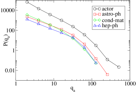
Figure 1: The actor degree distributions of the empirical data sets. All data appear to follow a power-law with exponent -1.6 for small $k$ but there is a noticeable cutoff in each set.

The degree distributions $P(q_{a})$ of the actors in the bipartite graph form are plotted in Fig. 1. Logarithmic binning is used to reduce the effect of statistical fluctuations. All the four data sets can roughly be fitted by a power-law degree distribution $P(q_{a})~{}\sim~{}q_{a}^{-\gamma_{a}}$ with $\gamma_{a}\approx 1.6$ in the low-$k$ region, but there is a pronounced high degree cutoff. This is very similar in all the cases considered.

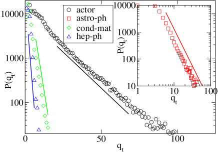
Figure 2: The tie degree distributions of the empirical data sets. The astrophysics collaboration network seems to exhibit a power-law distribution with the exponent being approximately -2.7. All the other data sets have an exponential decay. The solid straight lines are guides to the eye.

The degree distributions of the ties $P(q_{t})$ are depicted in Fig. 2. The movie–actor network data and the cond-mat and hep-ph scientist collaboration networks show an exponentially decaying degree distribution $P(q_{t})\sim e^{-q_{t}/q_{0}}$ with $q_{0}\approx 13.4$, $2.0$ and $1.0$ for the actor, condensed matter and high energy physics data sets, respectively. The astro-ph network is an exception since it clearly exhibits a power-law degree distribution for the ties (the inset of Fig. 2), i.e. $P(q_{t})\sim q_{t}^{-\gamma_{t}}$ with $\gamma_{t}\approx 2.7$. This would seem to point to the direction that the collaboration patterns in the astrophysics community differ essentially from those in other disciplines studied here. However, as seen below, most of the characteristic quantities of the networks are unaffected by such a different.

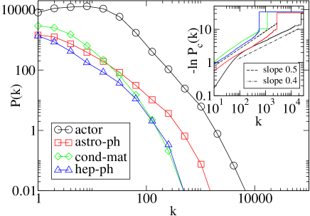
Figure 3: The degree distributions in the one-mode projection onto actors for the different empirical data sets as indicated by the legend. The scientist–article degree distributions are clearly not scale-free, but more reminiscent of the stretched exponential form (Eq. (9)) with $\alpha\approx 0.5$ as indicated in the inset. The movie-actor network appears to have a power-law scaling regime around $k=100$ but a more careful examination shows that the tail behavior is also of the stretched exponential form, now with $\alpha\approx 0.4$. The inset uses the same color coding for different data sets as the main figure.

The degree distributions in the one-mode projection onto actors are shown in Fig. 3. From the figure we see that the degree distribution of the actor-movie network has a lump in the lower-degree region, which is also somewhat visible in Fig. 2, and a short power-law region around $k=100$. However, a careful look reveals that the tail behavior follows the stretched exponential form

$$P(k)\propto k^{-\alpha}\exp(-\frac{\mu}{1-\alpha}k^{1-\alpha})\,,$$ (9)

where $\mu$ depends on $\alpha$ and satisfies $1\leq\mu\leq 2$ krapivsky:prl85 ; krapivsky:pre63 . For networks with this kind of degree distributions, the logarithm of the cumulative distribution function (shown in the inset of Fig. 3) is a power-law of the degree $k$. The inset clearly shows that this is the case here, and that in the scientist collaboration networks $\alpha\approx 0.5$ and in the actor network $\alpha\approx 0.4$. The observations made here about the degree distributions are compatible with previous studies ramasco:pre70 ; newman:pre64r .

III.3 Clustering and correlations

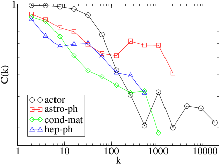
Figure 4: The $k$-dependent clusterings of Eq. (5) for the empirical data sets as indicated by the legend. It is worth noting that for small degrees $k$ the clustering is huge. The noisiness at high $k$ ($k>100$ for the scientist collaboration data, $k>1000$ for the actor data) comes from the low statistical quality of the data in these regions (cf. the degree distributions in Fig. 3).

The degree-dependent clusterings (naturally, in the one-mode projection) of Eq. (5) are plotted in Fig. 4, from which we see that the clustering is substantial (very close to one) for vertices with small degrees and gets lower with an increasing $k$. The low-$k$ behavior is expected since the actors with a small $k$ are likely to be connected only to collaborators sharing a single-tie, in which case the single-node clustering equals one. Furthermore, $C(k)$ is also expected to be monotonically decreasing because the more collaborators a node has the less probable it will be for those to be connected with each other.

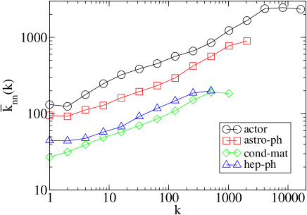
Figure 5: The average nearest-neighbour degrees (ANND) $\overline{k}_{nn}(k)$ as a function of the node degree $k$ for the empirical data sets. For each network, a power-law with exponent $\beta\approx 0.3$ can be roughly fitted to the data. This power-law behaviour is the most important empirical observation made here. Since the ANND is an increasing function of $k$, there is assortative mixing in the networks as typically in social networks.

The average nearest-neighbour degrees $\langle k_{nn}(k)\rangle$ (Eq. (2)) as a function of node degree $k$ are plotted in Fig. 5. All networks behave similarly with respect to this quantity; a power-law scaling

$$\overline{k}_{nn}(k)\sim k^{\beta}$$ (10)

with $\beta\approx 0.3$ is observed in each one, with some small deviations. At high degrees $k$ a cutoff, possibly a trace of the finite size of the networks, can be seen in each data set.

Since the ANND is an increasing function of $k$, one can conclude that significant assortative mixing is present in the network, i.e. the degrees of adjacent nodes are positively correlated. This can also be seen from the experimentally measured assortativity coefficient $r$ in Table 1. The differences in the amplitudes of the ANND curves in Fig. 5 are explained by the differences in the average degree $\langle k\rangle$ of the networks.

III.4 Preferential attachment

From the empirical data, the (one-mode) preferential attachment (PA) rule can also be measured quite straightforwardly given that the order of appearance (or preparation) of the articles or movies can be deduced from the available data, which is the case here. The measurement method has been devised by Newman newman:pre64r and goes as follows. Denote the degree-dependent preferential attachment rule, i.e. the bias to select actors of degree $k$, by $T_{k}$. Given such a rule, the time-dependent probability that a node added to the network at time $t$ connects to a node of degree $k$ is given by

$$P_{k}(t)=\frac{T_{k}n_{k}(t-1)}{N(t-1)}\,,$$ (11)

where $n_{k}(t-1)$ is the number of nodes with degree $k$ right before the addition of the new node and $N(t-1)$ is the total number of nodes in the graph at the same time. Given these quantities, the preferential attachment rule $T_{k}$ can be measured by making a histogram as a function of $k$ to which a new link is added with the weight of $N(t-1)/n_{k}(t-1)$ each time one is created.

If the attachment is non-preferential, $T_{k}$ is independent of $k$. On the other hand, with preferential attachment, $T_{k}$ is a growing function of the degree $k$ and for instance in the Barabási-Albert model barabasi:science286 $T_{k}\propto k$ by definition.

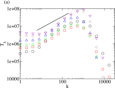
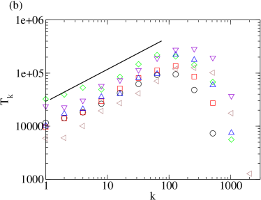
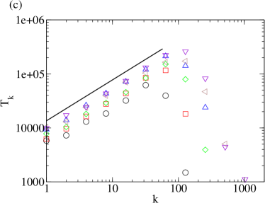
Figure 6: The measured effective preferential attachment (PA) rules for (a) the actor-movie network in the 1950s ($\circ$), 1960s ($\square$), 1970s ($\Diamond$), 1980s ($\vartriangle$), 1990s ($\vartriangleleft$) and 2000s ($\triangledown$), and for (b) the astrophysics, (c) the condensed matter physics and for (d) the high energy physics scientist–article networks during years 1998 ($\circ$), 1999 ($\square$), 2000 ($\Diamond$), 2001 ($\vartriangle$), 2002 ($\vartriangleleft$) and 2003 ($\triangledown$). The PA rules are well fitted by a power-law $T_{k}\sim k^{\alpha}$ with a cutoff and they appear to be independent of time. Numerically, we observe $\alpha\approx 0.65$ for the actor network, $\alpha\approx 0.6$ for the astrophysics network and $\alpha\approx 0.75$ for the other networks. The solid lines are guides to the eye.

The empirically measured PA rules are plotted in Fig. 6. All of them are well fitted by power-laws $T_{k}\sim k^{\alpha}$ with high-$k$-cutoffs. For the actor-movie network the measured value of the exponent $\alpha\approx 0.65$, for the astrophysics network $\alpha\approx 0.6$, and for the other networks $\alpha\approx 0.75$. Different decades (movies) or years (articles) of accumulation of the data are shown separately to illustrate that the effective PA rule is independent of time. Note that the amplitudes of the plotted curves are irrelevant, since $T_{k}$ is a relative probability. At low degrees ($k<10$) the behaviour of the actor data set differs from the other ones. In essence, $T_{k}$ is approximately constant in this region. This means that for low degrees the actual value becomes irrelevant and may perhaps indicate a sublinear version of Eq. (12). Note also that we have observed different exponents $\alpha$ for different data sets but the same numerical value of the ANND exponent $\beta$, effectively ruling out a direct connection between ANND and $T_{k}$.

The position of the cutoff increases as a function of time, and thus as a function of the network size. A similar cutoff can be observed when measuring the PA rule retroactively for a network generated numerically, so we conclude that the cutoff is merely a finite-size effect, which does not need to be taken into account explicitly while building a simulational model. Similarly, in the team assembly model, the retroactively measured PA rule is a power-law with a cut-off, but with $\alpha\approx 0.4$ and independent of the simulation parameters. We have not tried to consider the “$T_{k}$” for the tie one-mode projection, though it would naturally be of some interest.

Measurements of the preferential attachment rule in the arXiv.org collaboration networks were also reported in Ref. newman:pre64r by Newman. The measurement method used is the same as in this work. Surprisingly, Newman concludes that the preferential attachment is linear, which is in striking contrast to the results obtained here. Since the data sets and the measurement method are apparently the same, there remains only one possible explanation. Newman considered the arXiv.org network as a whole whereas in this work the division into disciplines is used. Also Barabási et al. barabasi:physicaa311 have measured the PA rule, but for different networks. They discover exponents 0.75 and 0.8 for neuro-science and mathematics scientist–article collaboration networks, respectively.

III.5 The one-mode projection onto ties

Figure 7: The degree distributions in the one-mode projection onto ties. The scientist-article networks have a region up to $k_{a}\approx 100$ where the probability density is practically a constant, followed by a rapid decay.

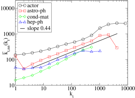
Figure 8: The average nearest-neighbour degrees in the one-mode projection onto ties. A common property of the scientist collaboration networks is an approximate power-law scaling.

The degree distribution and the average nearest neighbour-degree in the one mode projection onto social ties are shown in Figs. 7 and 8 respectively. The degree distributions in the scientist collaboration (article) networks are quite interesting. There is a practically constant region up to $k\approx 100$ and a relatively rapid fall at larger degrees. On the other hand, the movie network appears to behave differently. There is an approximate power-law with slope around $-0.6$ for small $k$ and no region of constant probability can be observed.

Analogously to the projection onto actors, the average nearest-neighbour degree approximately scales as a power of the degree $k$ also on this projection. The measured exponent is $\beta_{t}\approx 0.44$.

IV Previous models

Earlier studies of collaboration networks are mostly centered around unipartite networks, with a few exceptions ramasco:pre70 ; borner:pnas101 ; goldstein:cond-mat0409 ; guillaume:cond-mat0307 ; morris:cond-mat0501 ; barber:physics0509 . Growing unipartite networks are relevant to the present work since they tell how the degree distribution depends on the growth rule. E.g. if uniform attachment would be used, the degree distribution becomes exponential dorogovtsev:book , in contrast to a linear preferential attachment rule, with a power-law degree distribution barabasi:science286 . Between these two extremes lies sublinear preferential attachment, i.e. a network growth rule that states that a new node connects to an existing one with probability proportional to $k^{\alpha}$ ($0<\alpha<1$), where $k$ is the degree of the existing node. This kind of growth leads to a stretched exponential degree distribution of Eq. (9).

Another family of preferential attachment rules is given by attachment probabilities $\Pi_{k}$ of the form

$$\Pi_{k}\propto k+A\,,$$ (12)

where $A$ is a parameter also termed additional attractiveness dorogovtsev:book . This leads to scale-free networks with a tunable, $A$-dependent, degree distribution exponent $\gamma$. The networks develop degree correlations such that for $A>0$, $\overline{k}_{nn}(k)\sim\log(k)$ whereas for $A<0$, a decaying power-law $\overline{k}_{nn}(k)\sim k^{\beta}$ with $\beta<0$ is recovered barrat:cond-mat0410 .

The reference model is the bipartite configuration model newmanpark:pre68 ; guillaume:cond-mat0307 . In it, all actors and ties are created first, assigned degrees from given degree distributions and linked randomly such that the degrees are fulfilled. It has been proven mathematically newman:pre68 that this model always leads to a non-negative assortativity coefficient. Despite of this, the correlations are clearly too weak to explain those in the empirical data ramasco:pre70 .

Recently Ramasco et al. ramasco:pre70 have introduced a model of a growing bipartite collaboration network, which is defined as follows. At each time step, a new tie with $n$ actors is added to the network. Of these, $m(<n)$ are new, i.e. are not currently a part or the network. The rest $n-m$ are chosen from the set of pre-existent actors with probability proportional to the number of ties $q$ they have already participated in, i.e. by using linear preferential attachment. Ramasco et al. arrive at a scale-free degree distribution $P(k)\sim k^{-\gamma}$ in the one-mode projection onto actors with

$$\gamma=2+\frac{m}{n-m}\,.$$ (13)

While the model above can be solved analytically, it fails to explain some features when compared to empirical data ramasco:pre70 . The most important deviations are in clustering and correlations. To overcome this, Ramasco and co-workers introduced the aging of actors as an additional property of the model. In their model, the actors age such that the probability that an actor is alive (i.e. capable of participating in new ties) after having participated in $q$ ties is

$$P_{\mathrm{alive}}(q)=\left\{\begin{array}[]{lll}1&,&\mathrm{if}\;\;q<q_{0}\\ \exp\{-\frac{q-q_{0}}{\tau}\}&,&\mathrm{if}\;\;q\geq q_{0}\end{array}\right.\,.$$ (14)

There is a certain survival up to participation in $q_{0}$ ties and an exponential decay thereafter with a characteristic time $\tau$.

Introducing the aging renders the model analytically unsolvable and the degree distribution develops a cutoff at large values of the one-mode degree $k$. A similar cutoff is observed experimentally and Ramasco and co-workers use its position and steepness for determining the values of the aging parameters $q_{0}$ and $\tau$. With the aging one is able to make the assortativity coefficient (Eq. (3)) positive and increase the clustering coefficient (Eq. (7)) so that both get closer to empirically observed values.

Guimerá et al. guimera:science308 have introduced a model of team assembly mechanisms that is quite similar to the one discussed above. In their model, new teams are formed, and their members are selected according to the following rules. At each time step a new team with $m$ members is created. For each member an incumbent, that is a member that is already part of the network, is chosen with probability $p$, and a new one is created with probability $1-p$. If the previous member was an incumbent, the next one is selected from its collaborators with probability $q$, otherwise the selection is performed as above.

Identifying the teams with the social ties and the team members as the social actors, the team assembly model is a version of a growing bipartite network model. In it, the preferential attachment rule consists of two ingredients: The first incumbent member of each team and the subsequent ones with probability $1-q$ are selected with random attachment, whereas the rest are chosen using linear preferential attachment, which comes here into play implicitly since a random previous collaborator of a member is chosen holme:pre65 . Guimerá et al. have found that the degree distribution of the one-mode projection of the resulting graph mimicks empirically measured distributions reasonably well guimera:science308 .

Somewhat similar studies have also been conducted by Börner et al. borner:pnas101 , Goldstein et al. goldstein:cond-mat0409 and Morris morris:cond-mat0501 . A common goal of these is to introduce realistic models of collaboration networks. However, they do not pay any attention to degree-degree correlations. Similar ideas have also been applied to the bipartite network of research projects funded by the European Union and organizations participating in them barber:physics0509 .

V Sublinear model

Motivated by the empirical observations of the previous section, the following model of a growing bipartite collaboration network is proposed. It is also related to that of Ramasco et al. ramasco:pre70 (see also Sec. IV), but it is significantly modified in order for it to be consistent with empirical facts.

The model is as follows (the addition of a new tie is illustrated in Fig. 9).

• At each time step, a new tie is added to the network. The number of actors $n$ of this tie is a random variable whose distribution is given as an input parameter. Since this distribution can be measured experimentally, and the measured functional form is to be used, there is no fitting involved.

• Of these $n$ actors each one has a given probability $p$ to be a new one, i.e. at a fixed $n$ the number of new actors is a random variable with binomial distribution. The probability $p$ can be estimated from the data by selecting it such that, on the average, the total number of actors in the end of the simulation equals that in the empirical network being mimicked.

• The first one of the rest $n-m$ of them, with $m$ being the number of new actors, is chosen from the pool of all pre-existent actors such that actor $i$ gets chosen with probability

  $$p_{i}=\frac{k_{i}^{\alpha}}{\sum_{i}k_{i}^{\alpha}}\,.$$ (15)

  i.e. with sublinear preferential attachment. The corresponding rule of the model of Ramasco et al. has $\alpha=1$.

• Each one of the rest $n-m-1$ actors is chosen from the set of the earlier collaborators of the previously chosen actor with probability $p_{TF}$ also with sublinear preferential attachment, and as described in the previous point with probability $1-p_{TF}$.

Figure 9: An illustration of the one-mode projection and the addition of a new tie in the model with sublinear preferential attachment. Above the filled circles denote social ties, the open ones social actors and the lines the links between them. Below, each social actor is drawn again, now with links between them in the one-mode projection visible, i.e. two actors are connected if they participate in the same tie. (a) The network before the addition. For example, the leftmost actor has the bipartite degree $q_{a}=2$ and the one-mode projected degree $k=4$. Similarly, the leftmost tie has $q_{t}=3$ and $k_{t}=2$. (b) The network after the addition. The corresponding one-mode projections onto actors (ties) are drawn below (above) the bipartite networks. The new tie (the rightmost filled circle) introduced one new actor (the grey circle) who acquired two links to pre-existing actors (shown by blue lines). The new tie also caused a new connection between two pre-existing actors (shown by red line). The new tie connected to both existing ties; once to the leftmost one (one common actor) and twice to the middle one (two common actors). The same growth schematics also apply to the model of Ramasco et al. ramasco:pre70 and to the team assembly model guimera:science308 .

The most important new ingredient, the sublinear form of the PA rule, is justified by the measurements in Sec. III.4. Another quantum of motivation comes from the fact that degree distributions which are not pure power-laws have been measured (see Fig. 3 in Sec. III.2) and such degree distributions have been demonstrated to be caused by sublinear PA. Still further motivation is given by the studies of Onody and de Castro onody:physicaa336 where sublinear PA was found to lead to positive degree–degree correlations in terms of the assortativity coefficient $r$.

The motivation behind the triad formation (TF) process described in the last rule is the fact that several models incorporating this kind of behavior have been found to lead to increased clustering, closer to what has been observed in real networks holme:pre65 . A similar ingredient is also present in the team assembly model guimera:science308 , where the parameter $q$ plays the role of the triad formation probability.

VI Numerical results

network	empirical	sublinear	sublinear	team assembly
		$p_{TF}=0.0$	$p_{TF}=0.9$
$N_{a}$	28 526	25 497	24 650	24 477
$N_{t}$	49 330	49 000	49 000	49 000
$\langle q_{a}\rangle$	5.08	6.65	6.92	6.95
$\langle q_{t}\rangle$	2.94	3.46	3.48	3.47
$\langle k\rangle$	16.0	13.8	14.1	13.9
$\langle k_{t}\rangle$	56.3	36.1	107.6	33.2
$r$	0.250	0.13	0.15	0.26
$c$	0.370	0.10	0.18	0.32
$\overline{C}$	0.674	0.51	0.66	0.65

Table 2: The basic parameters of the simulated networks compared with the empirical condensed matter collaboration network.

In the simulations reported in this section, the number of ties in a simulated network is always $N_{t}=49000$, and the fraction of new social actors in a given tie is $p_{new}=0.202$. The same parameters are also used for simulations of the team assembly model, i.e.  $p=1-p_{new}$, and the simulation is run until $N_{t}$ teams are created. This selection of the parameters comes directly from the empirical measures of the condensed matter collaboration network. In the simulations of the team assembly model, the probability to select a previous collaborator of an incumbent is $q=p_{TF}=0.9$ unless otherwise mentioned. This choice leads to the correct order of magnitude in the clustering of the resulting graph, as will be seen below. In both models, the number $n$ of actors in a tie a drawn from the same probability distribution that corresponds to the empirically measured one (see Fig. 2). In addition, the aging mechanism is omitted in both models, i.e. the parameter $\tau$ of the team assembly model and the parameter $q_{0}$ of the model of Ramasco et al. are set to infinity. This appears to be justified since the ubiquitous characteristics of the ANND and the $k$-dependent clustering $C(k)$ do not show experimental dependence on the network age. Indeed, these are similar for both the movie network (in which aging surely has taken place) and the physics collaboration networks, in which the data collection is for a short interval and aging plays only a little role if at all. All the simulation results are from a single simulation run, i.e. from one network. To check the validity of this approach, we ran several simulations with the same parameters. The simulations are practically indistinguishable from each other, and thus we conclude that this is justified.

The basic parameters of the simulated networks, compared with the empirical condensed matter data, are shown in Table 2. The parameters that are either input to the models or straightforwardly depend on those, such as the number of nodes of different kinds, the average degrees in the bipartite network and in the one-mode projection onto actors, are, naturally, reproduced quite well. On the other hand, already the average degree $\langle k_{t}\rangle$ in the one-mode projection onto ties shows discrepancies between the simulations and the data. It appears that $p_{TF}$ could be used in the sublinear model to tune this value, but in this work the role of the tuning target is played by the average clustering $\overline{C}$. Regarding the clustering and correlations, the best numerical fit is given by the team assembly model.

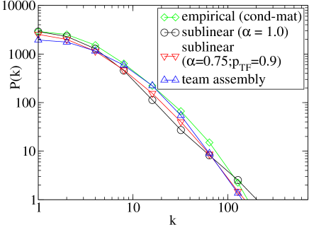
Figure 10: The degree distribution in the one-mode projection onto actors in the condensed matter collaboration network and in simulations of the sublinear model with different values of the PA exponent $\alpha$ and of the team assembly model with $p_{TF}$ = 1.0. The curve for $\alpha=1.0$ leads to power-law degree distribution as expected ramasco:pre70 , whereas that with $\alpha=0.75$ and the one of the team assembly model is clearly a lot closer to the empirical values. In the sublinear model, the behavior is the same even for $p_{TF}$=0 (not shown).

The degree distributions in the one-mode projection onto actors are plotted in Fig. 10 for the empirically measured condensed matter collaboration network and for simulations of the sublinear model with different values of $\alpha$ together with a simulation of the team assembly model. It is seen that the simulation of the sublinear model (with or without triad formation) with $\alpha$ equal to the experimentally measured effective one (Fig. 6) mimicks the empirical degree distribution significantly better than the one using the linear PA rule. The latter leads to a scale-free degree distribution as predicted ramasco:pre70 . Also the team assembly model is capable of reproducing the empirical degree distribution reasonably well. In the rest of this paper, the value $\alpha=0.75$ is used unless otherwise mentioned. Note that the comparison of the other networks studied empirically in this work to corresponding simulation yields the same behavior.

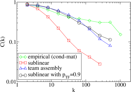
Figure 11: The $k$-dependent clustering (Eq.(5)) compared to empirical measurements for both the sublinear model ($\alpha=0.75$) and for the team assembly model. It is seen that the sublinear model at $p_{TF}=0$ cannot reproduce the clustering as expected whereas both the team assembly model and the sublinear model at $p_{TF}=0.9$ do somewhat better. However, not one of the models agrees fully with the empirical data.

The degree-dependent clustering $C(k)$ of Eq. (5) in the one-mode projection is plotted in Fig. 11 for the condensed matter collaboration network and for simulations both of the sublinear model and the team assembly model. From the figure, it can be seen that the sublinear model without triad formation differs notably from the empirical data whereas the sublinear model with a high probability for triad formation and the team assembly model give a correct order of magnitude for the overall clustering (see also Table 2) but the form of the $C(k)$ curve differs from the empirical one. In this respect, the sublinear model does slightly better that the team assembly model.

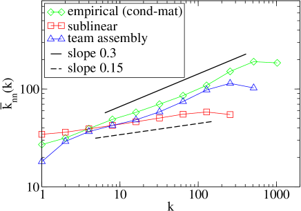
Figure 12: The average nearest-neighbour degree (ANND) in simulations of the sublinear model ($\alpha=0.75$) and the team assembly model compared to the empirical measurements. The results from the team assembly model are in reasonable agreement with the real data, whereas those from the sublinear one roughly scale as a power of $k$ but with a different exponent. The solid and dashed lines are guides to the eye.

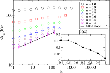
Figure 13: The average nearest-neighbour degree (ANND) in simulations using different values of the preferential attachment exponent $\alpha$. For all $\alpha$ the ANND scales as a power of the node degree $k$, $\overline{k}_{nn}(k)\sim k^{\beta(\alpha)}$ so that for $\alpha=1$, $\beta=0$, i.e. no degree-degree correlations are observed, and for $\alpha<1$, $\beta$ grows as $\alpha$ decreases leading to positive correlations. The inset shows the dependence of $\beta$ on $\alpha$.

The average nearest-neighbour degree $\overline{k}_{nn}(k)$ (ANND) is plotted in Fig. 12 for the condensed matter empirical data set and for simulations of both models. The figure shows that the team assembly model reproduces the correlation structure of the empirical network reasonably well in the intermediate-$k$ regime: both appear to roughly scale as $\overline{k}_{nn}(k)\sim k^{\beta}$ with $\beta=0.3$ and approximately agree in the amplitude. However, the simulation differs from the data at both low and high $k$-values. On the other hand, the simulations of the sublinear model show a similar scaling but with a different, smaller exponent ($\beta\approx 0.15$).

To study the effect of the exponent $\alpha$ on the scaling of the ANND in the sublinear model, it is depicted in Fig. 13 as a function of $\alpha$. For $\alpha=1$, we see that there are no degree-degree correlations at all, corresponding to the model of Ramasco and co-workers without aging. For lower values of $\alpha$, positive correlations are present and the ANND scales as a power-law of the vertex degree $k$ as above. The value of $\beta$ depends continously on $\alpha$ as seen in the inset of Fig. 13. However, the numerical value of the exponent $\beta$ is notably lower in the relevant region $0.6<\alpha<0.8$ than the experimentally observed one. Thus, the overall correlations in this case are not as strong as in the empirical data. This conclusion can also arrived at considering the values of the assortativity coefficient $r$ in Table 2.

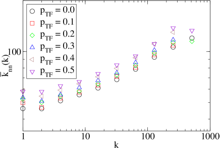
Figure 14: The scaling of the ANND for different values of the triad formation (TF) probability in simulations of the sublinear model. It is seen that introducing a TF mechanism does not change the scaling. In addition to the results in the figure ($\alpha=0.7$) we have checked this with several other values of $\alpha$, too, with the same results. The same also applies to the team assembly model (results not shown).

To see how to the triad formation affects the scaling of the ANND, it is plotted for several values of $p_{TF}$ in Fig. 14 for the sublinear model. It is clearly seen from the figures that the triad formation process has no effect at all. We have also performed a corresponding series of simulations with several different values of $\alpha$. In all cases, the conclusion remains the same. Simulations of the team assembly model also revealed the same behaviour. Thus, we conclude that this kind of process can not be held responsible for the observed correlations. Again, comparing the assortativity coefficient $r$ in Table 2 for the sublinear model with and without triad formation supports this conclusion.

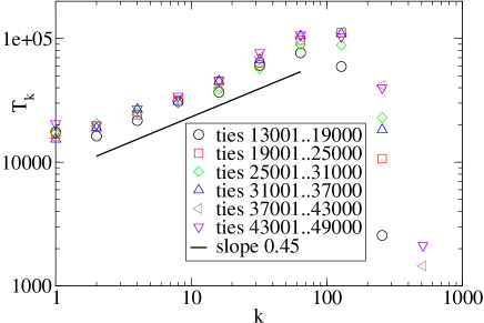
Figure 15: The retroactively measured preferential attachment rule for a simulation of the team assembly model. The rule is approximately a time-independent sublinear power-law with $\alpha\approx 0.45$ and with a cut-off. The solid line is a guide to the eye.

The retroactively measured preferential attachment rule for the team assembly model is plotted in Fig. 15. It is clearly seen that the rule is, again, a sublinear power-law with $\alpha\approx 0.4$ and with a cut-off that is very similar to the empirical ones (cf. Fig. 6) and to those in the simulations of the sublinear model (not shown). This is surprising since, at the first sight, one could anticipate that the combination of attachment rules in the team assembly model leads to a compound rule of the form $k+A$. However, the bipartiteness comes into play, and this phenomenon shows that it can indeed affect essentially the network structure. It can also be seen that the effective attachment rule is time-independent, as is true concerning the empirical data.

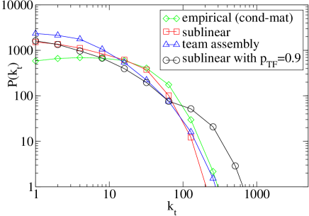
Figure 16: The degree distribution in the one-mode projection onto ties in the empirical condensed matter data set, compared to simulations. A considerable difference exists between the simulations and the data.

Figure 17: The average nearest-neighbour degree in the one-mode projection onto ties in the empirical condensed matter data set and in the simulations. These are unable to reproduce the empirically observed power-law scaling. Quantitatively, the team assembly model mimicks the behavior of the data better than the sublinear model.

Next we compare the models with the one-mode projection onto social ties instead of social actors. These are shown in Figs. 16 and 17 for the degree distribution and the average nearest-neighbour degree, respectively. From Fig. 16 one can see that the characteristic plateau of the scientist collaboration networks is not captured by any of the simulations. Similar conclusions can be made from Fig. 17: not one of the models lead to the power-law scaling that we have empirically observed. There are also considerable differences in the overall magnitudes of the quantities, in which respect the team assembly model behaves best.

VII Summary and discussion

In this paper, we have analyzed several bipartite collaboration networks empirically. The static and dynamic structure thereof is one of the conceptually simplest examples of complex networks, where effective statistical laws seem to exist. The quantitative description of such phenomena by models becomes then the (elusive) goal. These systems are very clear-cut in that the old graph structure is static - old vertices and edges are not removed - and that the growth events are easy to quantify by various measures and to follow, from data.

Concerning the correlation structure of collaboration networks, the most important empirical observation is that the average nearest-neighbour degree (ANND) in the one-mode projection onto social actors scales as a power of the node degree as $\overline{k}_{nn}(k)\sim k^{\beta}$ with $\beta\approx 0.3$. Similar scaling is also present in the projection onto social ties, i.e. articles or movies. The clustering of the one-mode network(s) is considerable. The effective actor-projection preferential attachment (PA) rule appears to be a sublinear power-law, and independent of time.

We have also introduced a model, which is built on top of this observation, in an attempt to explain the form of the observed properties of the networks. The empirically observed sublinearity of the PA rule has thus been included in a numerical model. In this case, the ANND indeed scales as a power of $k$, but the numerical values of the exponents do not match. In any case, the model is capable of demonstrating that the form of the PA rule can essentially affect the correlation structure.

Another model of team assembly mechanisms guimera:science308 has also been simulated. The ANND seems to fit the (actor) empirical observations reasonably well: both roughly scale as $k^{\beta}$ with $\beta\approx 0.3$. A common feature of both models is that they reproduce the degree distribution in the one-mode projection rather well (see Fig. 10). In the case of the sublinear model, using the correct, empirically measured, value of the exponent $\alpha$ is necessary for this result. On the other hand, team assembly model fails to reproduce the empiricál attachment rule.. The sublinear model without any triad formation fails to reproduce the form of the $k$-dependent clustering, whereas the team assembly model and the sublinear model with considerable probability for triad formation lead to correct order of magnitude of the average clustering $\overline{C}$, seen also in the overall magnitude of $C(k)$. However, the models do not explain its functional form. Note that a triad formation process does not change the correlations in the models studied here.

Considering the one-mode projection onto social ties instead of actors reveals the inadequacy of the both models. The empirically measured degree distribution and the average nearest-neighbour degree both differ from their simulated counterparts. In effect, we have observed that even though various can reproduce some properties of the projections onto actors, they lack explanatory power when it comes to considering the networks with their full bipartite structure intact. Perhaps one should consider tie-based growth rules instead of actor-based ones.

Summarizing, there is a clear need for a more complex bipartite growth model that accounts for both the clustering and correlations of actors (authors) and ties (articles). Since the bipartite structure changes by events in which one tie is introduced together with several actors, this means that the old actors’ effective choice must follow from a rule that measures the correlation structure in more detail. One candidate would be to use $k$-connected cliques in analogy to recent observations of the role of such in network superstructure palla:nature435 . This would allow for various ways of measuring the joint strength of interaction between old actors. Furthermore, using the recently introduced concept of social inertia ramasco:physics0509 might be of use in this respect, by establishing a quantitative time-dependent measure. It is also clear that there are substructures within subfields. These point towards the idea that the actors and ties have “hidden variables” that should be taken into account. One practical prospect would be to use e.g. the PACS indices to classify ties (articles) and actors/authors, and investigate the role of the both above ideas. Note that in all the cases here the “invisible college” or giant component of the one-mode projection onto actors includes really almost all of the actors and is thus trivial. It is an open question how to define and measure the “success” of an actor given this, and the performance of current models - simple membership is not enough. Again, possibly progress could be made by the use of weighted networks.

Even though several sources of positive degree-degree correlations have been demonstrated here, there are still open questions related to these. Most importantly, the reason or origin of the specific form of the correlations remains unknown. Perhaps one needs to define more informative quantities for measuring the structure of the original bipartite network. Studies on how the form of the (one-mode) PA rule depends on the underlying elementary social phenomena offer interesting avenues for future work.

Acknowledgments. We thank Sergey Dorogovtsev for numerous stimulating and useful discussions, and for a critical reading of an early version of this manuscript. This work was supported by the Academy of Finland, Center of Excellence program.

References

- (1) S. N. Dorogovtsev and J. F. F. Mendes, Evolution of Networks: From Biological Nets to the Internet and WWW (Oxford University Press, Oxford, 2003).
- (2) S. N. Dorogovtsev and J. F. F. Mendes, Adv. Phys. 51, 1079 (2002).
- (3) M. E. J. Newman, SIAM Review 45, 167 (2003).
- (4) R. Albert and A.-L. Barabási, Rev. Mod. Phys. 74, 47 (2002).
- (5) R. Pastor-Satorras, A. Vázguez, and A. Vespignani, Phys. Rev. Lett. 87, 258701 (2002).
- (6) M. E. J. Newman, Phys. Rev. Lett. 89, 208701 (2003).
- (7) A. Vázguez, R. Pastor-Satorras and A. Vespignani, Phys. Rev. E 65, 066130 (2001).
- (8) M. E. J. Newman, Phys. Rev. E 67, 026106 (2003).
- (9) M. E. J. Newman, Phys. Rev. E 68, 036122 (2003).
- (10) P. Holme and B. J. Kim, Phys. Rev. E 65, 026107 (2003).
- (11) J.-L. Guillaume and M. Latapy, e-print, cond-mat/0307095.
- (12) M. Boguña, R. Pastor-Satorras, A. Diaz-Guilera, and A. Arenas, e-print, cond-mat/0309263.
- (13) M. Boguña and R. Pastor-Satorras, Phys. Rev. E 66, 047104 (2002).
- (14) M. Boguña, R. Pastor-Satorras, and A. Vespignani, Phys. Rev. Lett 90, 028701 (2003).
- (15) R. Guimerá, B. Uzzi, J. Spiro, and L. A. N. Amaral, Science 308, 607 (2005).
- (16) J. J. Ramasco, S. N. Dorogovtsev, and R. Pastor-Satorras, Phys. Rev. E 70, 036106 (2004).
- (17) S. N. Dorogovtsev, Phys. Rev. E 69, 027104 (2004).
- (18) The Internet Movie Database, http://www.imdb.com/.
- (19) http://www.nd.edu/~networks/database/index.html.
- (20) arXiv.org e-Print archive, http://www.arxiv.org/.
- (21) A.-L. Barabási, H. Jeong, Z. Néda, and E. Ravasz, Physica A 311, 590 (2002).
- (22) P. L. Krapivsky, S. Redner, and F. Leyvraz, Phys. Rev. Lett. 85, 4629 (2000).
- (23) P. K. Krapivsky and S. Redner, Phys. Rev. E 63, 066123 (2001).
- (24) M. E. J. Newman, Phys. Rev. E 64, 025102(R) (2001).
- (25) A.-L. Barabási and R. Albert, Science 286, 509 (1999).
- (26) K. Börner, J. T. Maru, and R. L. Goldstone, Proc. Natl. Acad. Sci U. S. A. 101, 5266 (2004).
- (27) M. L. Goldstein, S. A. Morris, and G. G. Yen, e-print, cond-mat/0409205.
- (28) S. A. Morris, e-print, cond-mat/0501386.
- (29) M. J. Barber, A. Krueger, T. Krueger, and T. Roediger-Schluga, e-print, physics/0509119.
- (30) A. Barrat and R. Pastor-Satorras, Phys. Rev. E 71, 036127 (2005).
- (31) M. E. J. Newman and J. Park, Phys. Rev. E 68, 036122 (2003).
- (32) R. N. Onody, and P. A. de Castro, Physica A 336, 491 (2004).
- (33) G. Palla, I. Derényi, I. Farkas, and T. Vicsek, Nature 435, 814 (2005).
- (34) J. J. Ramasco and S. A. Morris, e-print, physics/0509427.