A modelling approach towards Epidermal homoeostasis control

Abstract

In order to grasp the features arising from cellular discreteness and individuality, in large parts of cell tissue modelling agent-based models are favoured. The subclass of off-lattice models allows for a physical motivation of the intercellular interaction rules.

We apply an improved version of a previously introduced off-lattice agent-based model to the steady-state flow equilibrium of skin. The dynamics of cells is determined by conservative and drag forces, supplemented with delta-correlated random forces. Cellular adjacency is detected by a weighted Delaunay triangulation. The cell cycle time of keratinocytes is controlled by a diffusible substance provided by the dermis. Its concentration is calculated from a diffusion equation with time-dependent boundary conditions and varying diffusion coefficients. The dynamics of a nutrient is also taken into account by a reaction-diffusion equation.

It turns out that the analysed control mechanism suffices to explain several characteristics of epidermal homoeostasis formation. In addition, we examine the question of how in silico melanoma with decreased basal adhesion manage to persist within the steady-state flow-equilibrium of the skin. Interestingly, even for melanocyte cell cycle times being substantially shorter than for keratinocytes, tiny stochastic effects can lead to completely different outcomes. The results demonstrate that the understanding of initial states of tumour growth can profit significantly from the application of off-lattice agent-based models in computer simulations.

I Introduction

I.1 Methodology

In many applications of mathematical modelling, continuum equations are used to describe the evolution of discrete biological systems such as tumours, epithelia, animal populations murray2002a etc. Such equations can be solved comparably efficiently and have helped to understand many qualitative and quantitative features of tumour growth byrne2003b ; schaller2006a . In this modelling approach, the discrete cell numbers are approximated by continuous functions. However, the inclusion of discrete effects even in simple models may lead to qualitatively different results bettelheim2001 ; louzoun2003 . This problem becomes even more important when modelling the initial evolution of cancer, which is thought to originate within a single cell gatenby2003a . For systems containing a few cells of a certain species only, the mathematical foundations of approximating the species dynamics by a continuous distribution function are rather shaky, and especially for the complicated interactions between several cell species including birth and death processes, one may expect a qualitatively different behaviour to arise from agent-based approaches.

Within the class of agent-based (individual-based) models, cellular tissues are modelled as a set of strongly-interacting discrete objects. At present, it seems reasonable to consider the cell as the smallest entity in these models, though this is not stringent (compare e. g. the extended Potts model graner1992 ; turner2002 ). For agent-based models, the concept of the cellular automaton neumann1966 ; gardner1970 has proven very useful, since it allows to describe cells by simple interaction rules. Tumour growth for example has widely been modelled with cellular automata smolle1998a ; dormann2002 ; ferreira2002 . Most of the current agent-based models are implemented on a lattice. In models where a single lattice site is occupied by a single cell, volume-nonconserving events such as proliferation require far-reaching configuration changes on the lattice, which in such models comes along with rupture of ”intercellular bindings” on a large scale meineke2001 . This leads to the necessity of deriving effective interaction rules, which can often not be easily related to physical laws. Consequently, the avoided lattice artifacts often come at the price of ending up with parameters that principally cannot be determined by independent experiments and predictive power of the model is lost. A physical motivation for cell-cell interactions can be included by allowing for shape fluctuations. In lattice models, this can be achieved by increasing the resolution of the lattice (i. e., by representing a single cell by a variable number of lattice nodes as e. g. in the Potts model turner2002 or the hyphasma model meyer_hermann2004 ). Likewise, one can also in off-lattice models introduce further degrees of freedom per cell (such as e. g. the dynamics of the cell boundary as in weliky1990 ; weliky1991 ). However, especially in the realistic case with three spatial dimensions, such models with an increased resolution use a dramatically increased number of dynamic variables and thereby the necessary calculation time increases (for example, in cickovski2005a about 13000 cells are considered with about 120 lattice nodes per cell in a three-dimensional setup). As an advantage however, physically-motivated interactions can be used to calculate the cellular dynamics. Off-lattice centre-based models drasdo1995 ; dallon2004 allow for physical interactions to be included without the disadvantage of the large number of dynamic variables. As a drawback, they assume an intrinsic cellular equilibrium shape (e. g. spherical or ellipsoidal) and treat all deviations from this form as small perturbations. Thus, they represent a compromise between speed of numerical calculation and model accuracy.

We have previously applied an off-lattice centre-based model to the qualitatively simple problem of multicellular tumour spheroid growth schaller2005a . In comparison to an analogous continuum approach schaller2006a it turned out that agent-based models have greater potential to describe specific biological systems realistically. Keeping in mind that continuum models also arise from averaging (thereby deleting information), this is not a big surprise. However, it must be said that the degree of model complexity should always be limited by the experimental signature and for many experimental signatures continuum models will suffice.

In this article, we set up an off-lattice centre-based model for the epidermis that is intrinsically consistent and is also based on physical interactions as far as possible. This has the advantage that the model can be falsified.

I.2 The Epidermis

The epidermis is a stratified squamous epithelial tissue. It does not contain separate blood vessels and is therefore dependent on diffusion of nutrients from the dermis situated below. The epidermis can be divided into several layers montagna1992 :

The innermost stratum germinativum or stratum basale (basal layer) is a monolayer, in which most cell divisions occur. It is separated from the dermis below by a basal membrane. A fraction of the cells created there by cell division travels upwards into the stratum spinosum. Within this layer, the process of cornification begins: The cytoplasm looses water and is filled with keratin filaments. Within the stratum granulosum, cells die off and their shape flattens. This special pathway of cell death is also called anoikis. Completely cornified cells mark the stratum corneum, which is clearly distinguishable from the layers below. This layer does not contain viable cells and constitutes an efficient barrier for water and many of its solutes. The thickness of this layer varies strongly for different regions of the skin montagna1992 . In the upper part of this layer, the cellular material detaches by dissolving intercellular contacts.

Within this article, only three layers will be distinguished: The term stratum medium will be used as a combination for all layers not belonging to the stratum germinativum or the stratum corneum.

The cell types encountered in the epidermis are keratinocytes, melanocytes, Langerhans cells, and Merkel cells. Of these, the dominant fraction is constituted by the keratinocytes with roughly 75000 cells per square mm hoath2003 ; bauer2001 .

Keratinocytes are produced in the stratum germinativum by cell division. In order to maintain epidermal homoeostasis, in average one of the two daughter cells must leave the basal layer and travel upwards. The keratinocyte remaining in the basal layer will be termed stem cell in this article. The cell travelling upwards transforms into a fully-differentiated keratinocyte – possibly undergoing transit amplifying proliferations barthel2000 – and reaches the surface after about 12 to 14 days. During this passage, the keratinocytes follow the process of cornification described above.

Melanocytes are dendritic cells that are distributed within the basal layer, and their density is approximately 2000 cells per square mm montagna1992 ; moncrieff2001 ; hoath2003 . They adhere to the basal membrane via hemi-desmosomes. Their normal function is to provide keratinocytes in the skin with melanin. Tumours arising from cancerous melanocytes are called melanoma. Since most cancerous melanocytes still produce melanin, such tumours have a characteristic black colour.

The Langerhans cells are dendritic cells of the immune system and it is believed that Merkel cells play a role in sensation. Since neither effects of the immune system nor the mechanisms of sensation will be studied here, the latter two cell types will not be contained in the in silico representation and will not be discussed further.

The diffusional properties of the skin have important implications on medication applied to this tissue. With an observed strong increase of the manifestation of melanoma moncrieff2001 , studies of melanoma development are of huge importance. Especially their early diagnosis bears the potential to improve the chances of recovery. Within this article, some basic questions related to the initial stages of melanoma growth will be addressed.

II The model

In view of the complicated matter in reality, any model will inevitably simplify the system by neglecting properties that we consider to be less important. Starting from this perspective, the following approximation may seem reasonable:

Within the model, cells are represented as adhesively and elastically interacting (compressible) spheres of time-dependent radii. Processes such as cell proliferation and cell death correspond to insertion or removal of spheres to the system, respectively. The cell growth determines the time-dependent cell radii. Accordingly, cells consume nutrients and their presence also changes the diffusive properties within the tissue. In analogy to the cell cycle, the model cells can assume different internal states.

Note that the simplifying assumption of spherical cell shapes facilitates the use of adjacency detection algorithms such as the Delaunay triangulation schaller2004 . The basic specifics and consequences of this paradigm will be examined in the following, whereas the detailed technical discussion can be found in the appendix.

II.1 Continuous model variables

The problem of describing the dynamics of cell-cell contacts is currently not solved. In this article we have chosen the Johnson-Kendall-Roberts (JKR) model johnson1958 ; johnson1971 – supplemented with viscous shear and normal forces and delta-correlated random forces. The JKR model includes elastic and adhesive normal forces and has been experimentally verified for soft materials such as rubber. The simultaneous treatment of elastic and adhesive properties goes beyond some previous modelling approaches kreft2004a ; picioreanu2004a ; schaller2005a . Cell movement within solution (and even more in tissue) can be regarded as highly overdamped, which is why viscous effects cannot be neglected (in fact, they are known to be dominant). A detailed discussion of these interactions can be found in appendix A for the JKR-model, appendix B for the random forces, and appendix C for the arising equations of motion including dampening force contributions.

Under the assumption of dominant friction and neglecting the contribution of torque to dampening, the equations of motion for $N$ cells can be written as a large $3N\times 3N$ matrix $A(t)$ acting on the $3N$-dimensional cell position vector $\mbox{\boldmath$x$}=\left[x_{1}(t),y_{1}(t),z_{1}(t),\ldots,x_{N}(t),y_{N}(t),z_{N}(t)\right]$

$$A(t)\dot{\mbox{\boldmath$x$}}=\mbox{\boldmath$b$}\,,$$ (1)

where the vector $\mbox{\boldmath$b$}(t)$ on the right hand side includes all non-viscous forces and the matrix $A(t)$ contains the dampening contributions, see also the example in the appendix D. Since there is no analytic form of these quantities, equation (1) has to be solved numerically.

As the friction matrix $A(t)$ has neither a diagonal (non-isotropic friction) nor another simple structure, its inverse cannot be easily calculated. The fact that only cells in contact can contribute to friction however leads to a sparse population of the dampening matrix. In addition, since more than one spatial dimension is considered, the dampening matrix is not even block diagonal. Therefore, the inverse of such a sparse matrix is not necessarily sparse as well and for the systems considered in this paper, the inverse matrix of $A(t)$ would even not fit into main memory of normal PC’s. Therefore, we have used an iterative procedure – the method of conjugate gradients, see appendix D – that does not necessitate the explicit calculation of $A^{-1}(t)$ to solve above equation for the position vector $\mbox{\boldmath$x$}(t)$.

In addition, one has to solve the problem of the dynamics of diffusible signals such as e. g. nutrients. If processes such as convection and flow transport are comparably small, these are well described by reaction-diffusion equations. Such types of equations arise naturally from the continuum equation, if one assumes that the flow is always proportional to the concentration gradient and tends to even out all gradients. The discretisation of reaction-diffusion equations on a regular lattice leads to a large linear systems as above. However, in this case the matrix possesses more symmetry properties and well-adapted algorithms exist for the solution, see appendix D. Note that an alternative approach circumventing a grid discretization would be to use the method of Green functions following newman2004 .

Within the JKR model, adhesion is described by an adhesion energy density parameter $\sigma$. Assuming spatially uniform receptor ($C_{i}^{\rm rec}$) and ligand ($C_{i}^{\rm lig}$) densities on the cell membranes of cells $i$ and $j$, this parameter can be expressed as $\sigma_{ij}=\frac{\sigma^{\rm max}}{2}\left[C_{i}^{\rm rec}C_{j}^{\rm lig}+C_{i}^{\rm lig}C_{j}^{\rm rec}\right]$, where $\sigma^{\rm max}$ determines the maximum adhesion energy density (model parameter). A measure for the total cellular binding strength can then be derived from the sum of all binding energies with the next neighbours

$$\Sigma_{i}(t)=\sum_{j\in{\cal NN}(i)}\sigma_{ij}(t)A_{ij}(t).$$ (2)

Assuming that cells with low binding are shed off the skin surface, we remove necrotic and cornified cells from the simulation as soon as their binding strength falls below a critical value $\Sigma_{i}\leq\Sigma^{\rm min}$ (model parameter). Note that this choice also has the consequence that non-viable cells without contact to other cells are also removed from the simulation. These cells do not have anchorage and would be shed off in the realistic epidermis. In the case of cornified and necrotic cells we have assumed an exponential decay of receptor and ligand molecules with a given rate $\alpha$, i. e.,

$$\dot{C}_{i}^{\rm rec/lig}=-\alpha C_{i}^{\rm rec/lig}\,.$$ (3)

In the JKR model [compare equation (8)], the resulting decreased cell-cell adhesion would – with unchanged elastic parameters – lead to a perturbation of the equilibrium distance. Therefore, we have chosen to adapt the elastic cell modulus simultaneously. To maintain for similar cells a constant equilibrium distance, this implies a decreasing elastic modulus according to

$$\dot{E}_{i}=-2\alpha E_{i}\,.$$ (4)

Although the loss of receptors and ligands as well as decreasing cell elasticity may be reasonable assumptions for cornified and necrotic cells, the overall time course may be quite different in reality. We have tried other forms of necrotic cell removal. For example, one could think of removing non-viable cells randomly at a constant rate as was done in schaller2005a . This possibility however did significantly disturb the layered structure of the stratum corneum. Holes in this protective layer in turn did lead to sudden loss of the proliferation-moderating soluble substance in the epidermis and thereby to irregular proliferative behaviour and considerable oscillations in epidermal thickness. The same problem occurred when assuming a (Gaussian-distributed) cell-specific time after which non-viable cells were removed from the simulation.

Thus, the assumptions regarding continuous model variables can be summarised as follows:

• cell shape : spherical with slight perturbations

• cell-cell interactions : elastic, adhesive, and viscous non-isotropic dampening

• approximations : dominating friction and neglect of the back-reaction of angular velocities on the kinetics

• necrotic and cornified cells : loss of receptor and ligands leading to a reduced intercellular adhesion

II.2 Discrete Model Variables

Without representations of internal cellular states, the model would merely calculate the mechanical interaction between a number of adhesively and elastically interacting deformable spheres. However, it is well known that the different states in the cell cycle yield a different cell behaviour. This should also be reflected in the model. Extending a previous agent-based modelling approach schaller2005a to the necessities of the epidermis, we distinguish between the following internal states in the model: M-phase, $\rm G_{1}$-phase, $\rm S/G_{2}$-phase, $\rm G_{0}$-phase, necrotic, cornified. The first four states are illustrated in figure 1 left panel.

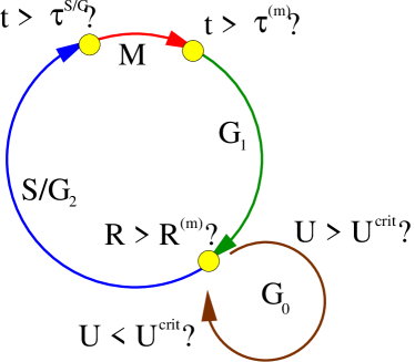
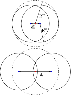
Figure 1: Left: Model realization of the cell cycle. During cell division, cells reside in the M-phase for $\tau^{\rm(m)}$. Afterwards, the cell volume increases at a constant rate in the $\rm G_{1}$-phase, until the pre-mitotic radius $R^{\rm(m)}$ has been reached. At the end of the $\rm G_{1}$-phase, the cell can either directly continue with the cell cycle or it can prolong the cycle time by entering the $\rm G_{0}$-phase, if the local concentration of the regulative substance (e. g. mobile water) exceeds a threshold $U^{\rm crit}$. The $\rm G_{0}$-phase is left after an individual time drawn from a Gaussian distribution or if the local concentration of the regulating signal falls below the critical threshold. Depending on the local nutrient concentration, cells can enter necrosis at any time in the cell cycle (not shown). In addition, keratinocytes enter anoikis in the fourth cell generation after completion of the $\rm S/G_{2}$-phase. Top right: Displayed is the configuration right at cell division at the beginning of the M-phase. The radii of the daughter cells (solid circles) are reduced to ensure conservation of the target volume. Bottom right: At the end of the M-phase, the daughter cells have relaxed. Due to interaction with neighbouring cells (not shown), the direction of mitosis may generally change during M-phase. An adaptive timestep in the numerical solution ensures that contact is maintained.

During $\rm G_{1}$-phase, the cell volume grows at a constant rate $r_{\rm V}$, i. e., the radius increases according to $\dot{R}=\left(4\pi R^{2}\right)^{-1}r_{\rm V}$, until the cell reaches its final mitotic radius $R^{\rm(m)}$. The volume growth rate $r_{\rm V}$ is deduced from the minimum observed cycle time $\tau^{\rm min}$ and the durations of the $\rm S/G_{2}$-phase and the M-phase. Afterwards, no further cell growth is performed.

At the end of the $\rm G_{1}$-phase, a checkpointing mechanism is performed. At this checkpoint, the cell can either enter the $\rm G_{0}$-phase or the $\rm S/G_{2}$-phase: In potten2000 it has been suspected that a diffusible substance produced at the basal layer might moderate the cellular proliferation. It is well known that the stratum corneum constitutes an effective barrier against the loss of water and its solutes as well as other substances barthel2000 ; bashir2001 ; kasting2003 . Its removal leads to a proliferative response. Hence, we use this correlation to establish a causal connection as a hypothesis. As the simplest model assumption, we will here assume the distribution of mobile water to influence cell proliferation. By mobile water we mean the fraction of the water content of the tissue that is not bound in intra- or extracellular cavities. Note that evidently the concentration of this water fraction can change in time and space. If the local mobile water concentration is below a critical value (model parameter), the cell will directly continue the cell cycle, whereas in the other case the cell cycle will be prolonged by the cell switching into the $\rm G_{0}$-phase. Cells leave the $\rm G_{0}$-phase to enter the $\rm S/G_{2}$-phase if either the local water concentration falls below the threshold or after an individual maximum time has passed (drawn from a random number generator, see subsection II.3). Note that the assumption of a different moderating diffusible signal would not significantly change the model as long as it is not created or consumed by the cells in the epidermis themselves.

Within this article the S-phase and $\rm G_{2}$-phase are not distinguished, their inclusion would be a mere technical aspect. After leaving the $\rm S/G_{2}$-phase (see subsection II.3), the cells deterministically enter mitosis. Keratinocytes and healthy melanocytes underly an exception at this point: After the fourth cell generation, keratinocytes cornify (enter anoikis) meineke2001 ; potten2000 ; barthel2000 . Healthy melanocytes simply remain at the end of $\rm S/G_{2}$-phase.

Within the model, the difference between the $\rm S/G_{2}$-phase and the $\rm G_{0}$-phase is that the duration of the first is determined by an individual duration that can be derived from experiments, whereas the duration of the latter is also controlled by the spatio-temporal evolution of the concentration of the moderating substance (in this case, mobile water).

One should be aware that our classification of internal cellular states may not directly correspond to the realistic biological system. However, the only net effect of the existence of the $\rm G_{0}$-phase is the prolongation of the cell cycle time: Cells in $\rm G_{0}$-phase can serve as a reservoir of cells ready to start proliferating as soon as the local water concentration falls below a critical threshold. A different terminology or a placement of the $\rm G_{0}$-phase after or within the $\rm S/G_{2}$-phase would therefore not significantly change the model.

At the beginning of the mitotic phase – which lasts for about half an hour for most cell types – a mother cell is replaced by two daughter cells. The radii of the daughter cells are decreased $R^{\rm(d)}=R^{\rm(m)}2^{-1/3}$ to ensure conservation of the target volume during M-phase. In addition, they are placed at distance $d_{ij}^{0}=2R^{\rm(m)}(1-2^{-1/3})$ to ensure that in this first discontinuous step the daughter cells do not leave the region occupied by the mother cell, see figure 1 right panels. In most cases, the daughter cells have the same cell type as the mother cell. The only exception is given by the keratinocyte stem cells which divide asymmetrically: By model assumption the upper daughter cell differentiates to a keratinocyte. The new cells are subject to their initially dominating repulsive forces (8). Note that an adaptive timestep derived from a maximum spatial stepsize ensures that the mitotic partners do not loose contact. Afterwards, the daughter cells enter the $\rm G_{1}$-phase thus closing the cell cycle.

Viable cells can enter necrosis at any time in the cell cycle as soon as the nutrient concentration at the cellular position falls below a cell-type specific critical threshold (model parameter). As the dominant pathway to cell death, keratinocytes in contrast enter anoikis after completing $\rm S/G_{2}$-phase in the fourth generation. Naturally, necrotic or cornified cells do not consume any nutrients.

The corresponding assumptions on discrete model variables can be summarised as follows

• cell proliferation

  • cellular states: M-phase, $\rm G_{1}$-phase, $\rm S/G_{2}$-phase, $\rm G_{0}$-phase, necrotic, cornified

  • local mobile water concentration can prolong the duration of $G_{0}$ state for keratinocytes

  • conservation of target volume during M-phase

  • for stem cells: upper cell differentiates to a keratinocyte, lower cell remains a stem cell

  • keratinocytes can undergo a maximum of four transit proliferations, whereas stem cells divide ad infinitum

  • healthy melanocytes do not proliferate, whereas malignant melanocytes can divide ad infinitum

• cell growth: growth of cell volume at constant rate during $\rm G_{1}$

• cell death

  • low local nutrient concentration induces necrosis

  • keratinocytes undergo cornification after fourth generation

  • cornified cells without contact to others are removed from the simulation immediately

II.3 Stochastic Elements

It is an empirical fact that processes in biological systems underly significant stochastic deviations: For example, biofilm cell populations starting from a single cell desynchronise proliferation after about five generations kreft1998 . Such a behaviour can not be explained by processes such as contact inhibition or nutrient depletion, as these are not active for small systems with only $2^{5}$ cells.

In the model, this is represented by stochastic elements that can be derived from a pseudo-random number generator matpack_manual . The involved stochastic elements are the delta-correlated random forces (see appendix B) acting on every cell, the initial direction of the displacement vector at mitosis, and the durations of some cell cycle phases such as the M-phase, the $\rm S/G_{2}$-phase, and the $\rm G_{0}$-phase.

As was done in previous models for biofilms kreft2001a ; picioreanu2004a , the initial direction of mitosis is determined from a random distribution, which is unifom on the unit sphere. This is the simplest modelling assumption that did not induce artifacts. In addition, it should be noted that during M-phase configuration changes are still possible due to interactions with the neighbouring cells.

In order to yield a sufficiently fast desynchronisation of the cell cycles, the individual duration times for the M-phase and the $\rm S/G_{2}$-phase as well as the maximum duration time for the $\rm G_{0}$-phase are drawn from a normally-distributed random number generator matpack_manual with a given mean and width. Without these stochastic elements, the model exhibits artificial oscillations around a steady state even in later stages. Technically, the duration of each phase is determined at the beginning of the phase. Naturally, the parameters on the random number generators can be set individually for every cell type.

II.4 Computer Platform

The computer code was written following the paradigm of object-oriented programming in $\rm C^{++}$ and was compiled with the GNU compiler gcc version 3.3. The code was executed on an AMD Athlon(tm) MP Processor 1800+ with 1 GByte of RAM on a Linux platform.

II.5 Simulation setup

As the computational domain, a rectangular box of dimensions $\rm 200\;\mu m\times 200\;\mu m\times 400\;\mu m$ has been considered. Since epidermal tissue is anisotropic, the boundary conditions have to be chosen non-homogeneous as well. Note that the cellular kinetics is described with a system of ordinary differential equations (26). Therefore, the term “boundary condition” refers to the special interactions of cells with the boundary of the computational domain. It is known that a realistic epidermis exhibits a ruffled basal layer montagna1992 . However, in order to treat the microenvironment of epidermal tissue as simple as possible, the basal layer has been implemented here as a static planar boundary at the bottom with normal vector $\mbox{\boldmath$e$}_{z}$. With using the JKR model (8), the interaction with such a planar boundary can be well implemented by assuming contact with a cell of infinitely large radius. Specifically, the $z$-boundary has been assumed to be of infinite elasticity $E_{\rm bound}=\infty$. Since the inverse elastic moduli enter additively in the JKR model in equation (6), this choice does not sensitively change the global model behaviour but merely shifts the equilibrium distance between basal membrane and bottom cell layer. The corresponding adhesive anchorage in the basal layer has been made dependent on the cell type (see the discussion below). In order to minimise the boundary effects in $x$ and $y$ direction, periodic boundary conditions could be used for the cell cell interaction. This however would necessitate a rather tedious mirroring of cells close to the boundary. In addition, one would have to use periodic boundary conditions on the associated reaction-diffusion equations as well to avoid additional artifacts. Therefore, here a different (mirror cell) approach has been chosen: Every cell in contact with a $x$ or $y$ boundary is assumed to be in contact with a cell of the same type, size, receptor and ligand equipment, etc. In short, it interacts with a virtual mirror copy of itself, where the contact area is situated within the boundary plane. In upper $z$-direction there are no boundary conditions on the cells – recall that necrotic or cornified cells are removed eventually. In comparison to a static boundary this procedure also has the additional advantage that drag force artifacts are reduced.

The boundary conditions on the cells have their counterpart in the reaction-diffusion equations for the mobile water concentration and the nutrients: The concentrations at the lower $z$-boundary have been fixed to the maximum value (Dirichlet boundary conditions), and above the cell layers (dynamic thickness, a stratum corneum need not always exist during the simulations) both concentrations are fixed to 0. Technically, this has been implemented by setting the concentrations to vanish at all grid volume elements not containing any cells: The resolution of the reaction-diffusion grid was low enough to prevent the emergence of artificial sink terms in intercellular cavities throughout all simulations (such problems could – in principle – also be avoided completely by using Green functions newman2004 ). At the $x$ and $y$ boundaries, no-flux von Neumann boundary conditions have been used, i. e., $\partial_{x}u=0$ and $\partial_{y}u=0$. Note that this is equivalent to the corresponding boundary conditions on the cells: The boundary is impenetrable for both cells and nutrients. Thus, for an in $x$ and $y$ directions homogeneous cell distribution, the problem would effectively reduce to a one-dimensional one.

The initial conditions have been determined as follows: A monolayer of keratinocyte stem cells was distributed on the basal membrane. Afterwards, the position of the cells in the cell cycle has been randomised uniformly to avoid initial artifacts. This configuration could for example mimic a severely perturbed epidermis, where suddenly not only the stratum corneum but also the stratum medium was removed. Consequently, a strong proliferative response should be expected.

After establishment of a steady-state flow equilibrium, different perturbations have been performed. These will be discussed in the next section.

III Results

III.1 Flow equilibrium

Our first question was whether the proposed control mechanism of the water-concentration-induced prolongation of the cell cycle time could actually produce the macroscopically observed flow equilibrium of skin. In particular, we asked whether

• a steady-state flow equilibrium is established, and

• whether this equilibrium is stable against perturbations such as complete removal of the stratum corneum that is performed for example in tape-stripping experiments barthel2000 .

These questions can be interpreted as a sanity check of the model assumptions and it turns out that both have an affirmative answer (see figure 2).

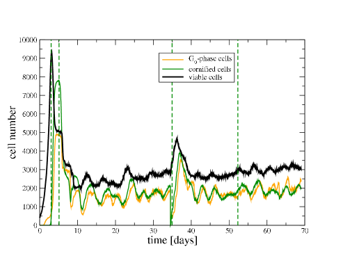
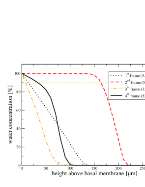
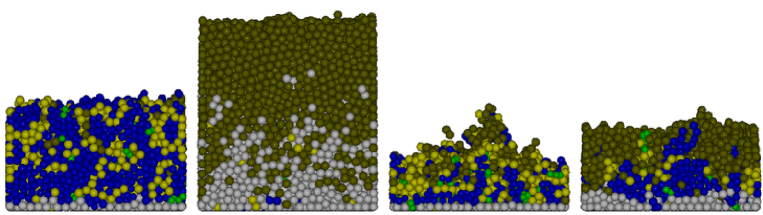
Figure 2: Emergence of an epidermal steady-state flow equilibrium. Top Left: Distribution of keratinocytes in the cell cycle. Cell numbers refer to a ground surface of $\rm 200\times 200\;\mu m^{2}$. Vertical dashed lines indicate times where cross-sections of the keratinocyte distribution (bottom row) and the water concentration (top right) have been extracted. Top Right: Shown is the (in $x$ and $y$ averaged) dependence of the concentration of mobile water on the distance from the basal layer at different times. The maximum value of 100 % corresponds to the mobile water concentration at the basal membrane and the horizontal dashed line denotes the critical mobile water concentration $U_{\rm H_{2}0}^{\rm crit}=90$ %. Bottom row: Shown is a cross-section in the $x-z$-plane of the in silico epidermis. Cells in $\rm G_{0}$-phase are marked in light grey, cornified keratinocytes are marked in grey, and darker shades of grey denote the different phases of the cell cycle. The first frame corresponds to an excited state already, whereas the last frame displays the flow equilibrium distribution predicting an approximate thickness of $120\;\mu m$ above the basal membrane.

Starting from a monolayer of cells, the local water concentration above the basal membrane is quite low such that no cell enters cell cycle prolongation. The net effect is an initial exponential growth phase (top left panel). After four generations, cornification of the first keratinocytes begins, followed by the formation of a stratum corneum with a considerably decreased diffusion coefficient for water. This in turn leads to an increased water concentration and thereby a greater fraction of cells residing in $\rm G_{0}$-phase: The initial exponential growth slows down and then the cell number decreases, since the cornified cells shed off the skins surface. Afterwards, the dynamics equilibrates. After 35 days, a tape-stripping experiment has been performed: All cornified cells are suddenly removed from the simulation. This leads again to a proliferative response. However, since this time the cornified layer quickly re-establishes due to reservoir cells in $\rm G_{0}$-phase, the proliferative response is considerably smaller than initially. Note that the dominant contribution to the rapid formation of the cornified layer in the model results from the fraction of $\rm G_{0}$-keratinocytes that have already reached their fourth generation. Interestingly, the oscillations around the equilibrium value are remarkably strong. The number of cells displays a slight (but decelerating) upward tendency, but 15 days after the disturbance (last vertical line), saturation is nearly reached. The final cell numbers correspond well to observed densities of keratinocytes (75000 cells per square mm skin at the breast bauer2001 ). In the top right panel of figure 2 it is demonstrated that with an intact stratum corneum (second and last frame), the water concentration is large in the lower layers of the epidermis and then falls rapidly. In figure 2 bottom row it becomes visible in the latest frame that the cornified layer exhibits a small hole (cells in dark grey). Due to a considerable loss of water, this causes many distant keratinocytes to leave their cell cycle arrest (cells in light grey changing to cells in dark grey) and thereby leads to a perturbation of the equilibrium.

In potten2000 the authors had hypothesised a diffusible substance that moderates cellular proliferation times. The present model does not contradict the hypothesis that this substance could simply be the moisture of the epidermis but other diffusible substances would presumably lead to equivalent model behaviour. Therefore, a confirmation/falsification of this model hypothesis would require more data on the candidate substances (diffusion coefficients, reaction rates, concentrations) and the associated processes.

III.2 Melanocyte anchorage

Another question is how the degree of anchorage to the basal layer influences the ability of cancerous melanocytes to persist within the skin. It is well-known that most human melanoma cell lines have decreased or no expression of cadherins and exhibit a decreased ability to adhere to keratinocytes tang1994 . Therefore, this question is especially interesting from a clinical point of view. At first, we suspected that increased basal adhesion would lead to an increased fraction of melanocytes bound to the basal membrane and thereby a smaller fraction that is shed to regions where the nutrient supply falls below necrosis-inducing levels. Thus, the total number of melanocytes should decrease with decreasing anchorage. In order to test this, a single (non-proliferating) melanocyte was placed at the basal layer in the centre of the computational domain, and the system was evolved until flow equilibrium was established. Then, the melanocyte was turned cancerous by suddenly allowing for proliferation with a much larger rate than keratinocytes. In addition, we concomitantly reduced the anchorage to the basal layer. Starting from experience with multicellular tumour spheroids schaller2005a , we assumed the cycle time of cancerous melanocytes to be in the order of 15 hours. Surprisingly, it turned out that the overall growth dynamics was hardly dependent on the anchorage to the basal layer, see figure 3 left panel. Initially, the growth of melanocytes follows an exponential growth law, which is soon slowed down since the melanocytes reach distant regions from the basal layer, where nutrient support is poor. Since due to nutrient depletion the total number of viable cells already indicates saturation, also the total number of melanocytes must saturate eventually. Even with no adhesion to the basal membrane, comparable numbers of tumour cells were produced. Direct observation of the cross-sections (not shown) revealed the reason: With the given melanocyte proliferation rate of 15 hours, exponential growth was always faster than the epidermal flow induced by the turnover on the basal layer.

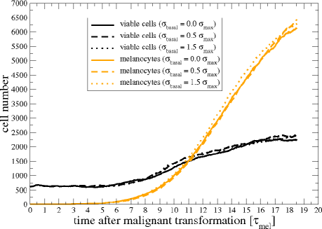
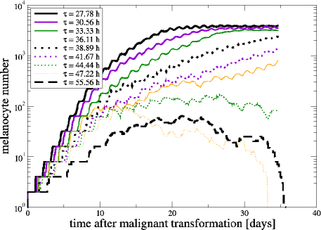
Figure 3: Left: Total number of melanocytes (grey, including necrotic and viable melanocytes) and viable cells (black, including stem cells, keratinocytes, and melanocytes) for different degrees of basal adhesion versus time – expressed in units of the cancerous melanocyte cycle time. For the assumed melanocyte cycle time of $\tau_{\rm mel}=(15.0\pm 2.0)$ h and other parameters chosen as in table 1, the basal anchorage has no significant effect on the overall dynamics. Right: With slower melanocyte proliferation and completely absent adhesion to the basal layer, a parameter regime can be found where melanoma do not persist within the steady-state flow equilibrium. Although melanocyte proliferation is still much faster than keratinocyte proliferation, the system is sensitive to stochastic effects, as is also indicated in the disturbed order (some curves intersect). The slowly-damped oscillations stem from the small standard deviations of melanocyte cell cycle durations (2 h in every run).

Consequently, we varied the proliferation rate of the cancerous cells in combination with complete loss of basal membrane anchorage (see figure 3 right panel). It turned out that there is a region of proliferation rates, where the melanocytes do not persist within the epidermis. This region is separated from the region of melanoma persistence by a comparably large domain where stochastic effects become important. Interestingly, in this case the period of coexistence of healthy skin and transformed cells may be remarkably long, which may give time for further malignant transformations in the realistic epidermis. It should be stressed that in this region the melanocyte proliferation rate is still much larger than the keratinocyte proliferation (their cycle prolongation is active for small melanoma). In addition, in the absence of death processes the growth law of keratinocytes follows the equation $\dot{n}_{\rm ker}=16\alpha_{\rm stem}n_{\rm stem}$, if one neglects the retardation induced by the four transient keratinocyte proliferations. This leads to linear growth only (with a fixed number of stem cells $n_{\rm stem}$), whereas the growth law of malignant melanocytes will be exponential $n_{\rm mel}=n_{\rm mel}^{0}e^{\alpha_{\rm mel}t}$ in the absense of death processes.

We further examined the region that separates melanoma persistence and complete shed-off of cancerous melanocytes by changing the melanocyte cycle time to $\tau_{\rm mel}=(44.44\pm 5.56)$ h. One finds that the usual spherical form one observes for in vitro tumour spheroids is considerably deformed for this system to cylinder-shaped or cone-shaped, compare figure 4 left panel. This is due to the pre-existent flow-equilibrium of the surrounding tissue and the effective one-dimensional diffusional constraint. Note also that the boundaries of the tumours are rather diffuse. Initially, a thin column of cancerous melanocytes is formed. Then, in the example in figure 4, left panel, first row, the melanocytes can persist within the life-sustaining zone until their growth velocity outweighs the upward-directed flow velocity and direct contact with the basal membrane is re-established. Afterwards, in the middle of the column of cancerous cells the upward forces are decreased, since for the interior cells there is no direct contact with keratinocytes moving upwards. In the simulations in figure 4 left panel, the thickness of the epidermis increases in those simulations where the tumour has re-established contact with the basal membrane. This is due to the displacement of keratinocytes – which are constrained in $x$ and $y$ dimensions – and also to the loss of the protective cornified layer, which leads to enlarged keratinocyte proliferation rates. It may be speculated that the cross-sections correspond to initial stages of a highly aggressive nodular melanoma moncrieff2001 that has not yet become clinically manifest. It may also be hypothesised that the micrometastases sometimes observed around primary melanoma in skin may correspond to branches of melanoma clones that have separated from the main clone during the upward flow. Interestingly, the shapes of these structures appear to be dynamically changing in these initial phases.

Using different initial seed values for the random number generator, we have performed several simulations with otherwise equal parameters. It turns out that completely different outcomes may occur in this region of melanocyte proliferation rates (figure 4 left panel and thick curves in the right panel). The stochastic effects result from stochastic forces, the randomly chosen mitotic direction, and the randomly distributed duration times of the cell cycle. In this in silico experiment, the different seed value did already lead to different configurations before the malignant transformation. More specific, the initial conditions for the growth of cancerous melanocytes had also been varied by employing stochastic elements before. In order to separate these effects, we started another series of simulations with equal initial seed values. In contrast to the previous simulations, the seed value of the random number generators was reset to different values right at the time of the malignant transformation. Thus, the initial environment of the cancerous melanocyte was the same in these simulations. It turned out that the variance of the outcomes narrowed considerably (thin grey curves in figure 4 right panel) but still exhibit large variations in the cell number (logarithmic plot). Thus, it can be concluded that the initial environment of cancerous melanocytes contributes significantly to the final outcome. Note that this does not only refer to the spatial cellular position, but also to the local proliferative state and thereby to the local upward flow velocity: The upward drag forces will be larger if the cancerous cell is surrounded by many proliferating keratinocytes with a net upward flow velocity.

In conclusion, stochastic effects generally play an important role in the initial phases of in silico melanoma development, since for the small cell numbers in the initial phases, they do not average out completely. In addition, their secondary consequences, i. e., the variation of the initial local environment by stochastic influences, are relevant.

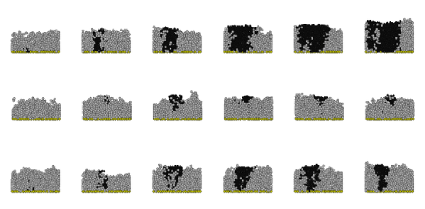
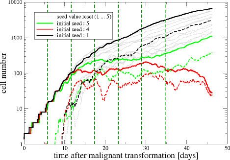
Figure 4: Left: In silico evolution of cancerous melanocytes (black) within an epidermal population containing keratinocytes (light grey) and stem cells (the bottom layer). The cross-sections do not distinguish between viable and necrotic or viable and cornified cells, respectively. The times at which the cross-sections have been produced are marked in the right panel with dashed lines. The first row corresponds to the seed value 1 (thick black curves in the right panel), the second row to seed value 4 (thick curves in grey), and the last row to seed value 5 (thick curves in light grey). Note that the diameter of a single frame is $200\rm\;\mu m$ only, such that the figure represents the state before clinical manifestation. Right: Total number of melanocytes (thick lines) and necrotic melanocyte subpopulation (associated dashed curves emerging around day 10) after the malignant transformation. For the thick lines, the different shades of grey correspond to different initial seed values (with otherwise equal parameters) of the random number generator. Consequently, these simulations also already include a changed environment for the melanocyte at the time of its malignant transformation. Note that for seed value 4 there are hardly any viable melanocytes left after 45 days (dashed and solid curves combine). This is different if the stochastic effects do not refer to the initial environment configuration of the cancerous melanocyte (thin curves in light grey).

IV Model parameters

Reasonable dynamics has been achieved with the parameters in table 1.

parameter	value	comment
ECM viscosity $\eta$	0.001 kg/($\mu$m s)	schaller2005a ; galle2005a
adhesion energy density $\sigma^{\rm max}$	0.0001 $\rm Nm/m^{2}$	chu2004
minimum anchorage $\Sigma^{\rm min}$	0.00001 pJ	estimate
receptor loss rate $\alpha$	0.00001/s	estimate
tangential friction coefficient $\gamma_{\parallel}$	0.1 $\cdot 10^{12}\rm Ns/m^{3}$	galle2005a
stochastic force coefficient $\xi$	0.001 $\cdot 10^{-6}\rm kg\;m/s^{3/2}$	D = 0.0001 $\rm\mu m^{2}/s$ schaller2005a ; galle2005a
M-phase duration $\tau^{\rm(m)}$	(1.0 $\pm$ 0.25) h	schaller2005a
$\rm S/G_{2}$-phase duration $\tau^{\rm(S/G_{2})}$	(5.0 $\pm$ 2.0) h	schaller2005a
keratinocyte $\rm G_{0}$-phase prolongation $\tau^{\rm(G_{0})}$	(138.9 $\pm$ 138.9) h	barthel2000
shortest observed keratinocyte cycletime $\tau^{\rm min}$	15 h	schaller2005a ; barthel2000
pre-mitotic cell radius $R^{\rm(m)}$	5.0 $\mu$m	norlen2004
cell elastic modulus $E_{i}$	750 Pa	mahaffy2000
cell Poisson ratio $\nu_{i}$	1/3	maniotis1997
melanocyte glucose uptake rate $\lambda^{\rm mel}$	150.0 amol/(cell s)	wehrle2000
keratinocyte glucose uptake rate $\lambda^{\rm ker}$	10.0 amol/(cell s)	estimate
critical water concentration $U_{\rm H_{2}0}^{\rm crit}$	90.0 %	kasting2003
maximum water concentration $U_{\rm H_{2}0}^{\rm bound}$	100.0 %	by definition
critical glucose concentration $U_{\rm gluc}^{\rm crit}$	1.0 mM	freyer1986a
water diffusivity $D_{\rm H_{2}0}^{\rm strat.med.}$	$1000.0\;\rm\mu m^{2}/s$	chenevert1991 ; livingston1995
water diffusivity $D_{\rm H_{2}0}^{\rm strat.corn.}$	$0.2\;\rm\mu m^{2}/s$	schwindt1998 ; bashir2001
glucose diffusivity $D_{\rm gluc}^{\rm tissue}$	$256.0\;\rm\mu m^{2}/s$	tuchin2001
glucose boundary concentration $U_{\rm gluc}^{\rm bound}$	5.0 mM	carvalho2004
stem cell basal adhesion energy density $\sigma^{\rm basal}$	$2\sigma^{\rm max}$	estimate

Table 1: Model parameters have been estimated from independent experiments or they have been varied as fit parameters. Parameters not included in the table have been also varied and are discussed in separate sections of this article.

The viscosity of the extracellular matrix $\eta$ determines the friction on loosely bound cells. Large viscosities lead to increased friction. Since viscous friction due to the cytoskeleton is assumed to be small ($\gamma_{\perp}\approx 0$, compare appendix C) – also dominates friction in directions normal to the cell contact surfaces. Thereby, also the initial speed of cell division in M-phase is dominantly dependent on $\eta$. As long as the force relaxation occurs on a shorter timescale than the total cell doubling time, this does not have macroscopic effects on the evolution of the tissue. This is different when $\gamma_{\perp}$ does not vanish. If it has the same order of magnitude as $\gamma_{\parallel}$, it will dominate the contribution inflicted by the viscosity $\eta$. However, if the magnitude of the total drag force coefficient does not change (marked by $\gamma^{2}=\gamma_{\perp}^{2}+\gamma_{\parallel}^{2}$), we have found by comparing the three extreme cases (that is, $\gamma_{\perp}=0,\gamma_{\parallel}=\gamma$ and $\gamma_{\perp}=\gamma,\gamma_{\parallel}=0$ and $\gamma_{\perp}=\gamma_{\parallel}=\gamma/\sqrt{2}$) that the differences in the overall population dynamics are rather small. It may be speculated that this is because in the present calculations the relaxation speed has no direct back-reaction on the number of cells, as in contrast to galle2005a ; schaller2005a contact inhibition has not been included in the model. As here absence of perpendicular friction has been assumed, the tangential friction coefficient $\gamma_{\parallel}$ dominantly determines the speed of relaxation within the tissue. The chosen value led to reasonable dynamics and has been estimated from galle2005a .

The adhesion energy density $\sigma^{\rm max}$ determines the cell-cell equilibrium distance and the binding strength, which was a marker for the removal of necrotic or cornified cells. Generally, this value will in reality be time-dependent, compare also the discussion at the end of subsection II.1. Therefore, the binding energy density has been derived from the observed equilibrium distance chu2004 solving (8) instead. With this procedure, the equilibrium distances are in a physiological regime. Note that larger adhesion will lead to smaller equilibrium distances (with moderately increased contact surfaces and drag forces) but also to longer persistence times of dead cells, which results in an increased thickness of the stratum corneum. However, due to equation (3) this latter effect only enters logarithmically. When both the adhesion energy $\sigma^{\rm max}$ and the minimum anchorage $\Sigma^{\rm min}$ are decreased, one will still have to decrease the maximum stepsize in the numerical solution to maintain the level of accuracy. This is due to the fact that for decreased adhesion, the equilibrium distance and the contact distance $d_{ij}^{\rm contact}=R_{i}+R_{j}$ are closer together.

The equilibrium thickness of the cornified layer is strongly dependent on the receptor loss rate $\alpha$ and the minimum anchorage $\Sigma^{\rm min}$. In addition, it will be sensitive to the cycle times of stem cells and keratinocytes, since these determine the number of keratinocytes finally undergoing cornification.

The elastic parameters correspond to approximate physiologic values for cells mahaffy2000 ; maniotis1997 ; galle2005a . However, it is known that – depending on the cell type and individual cytoskeleton – significant deviations may occur. With the given drag forces, mechanical relaxation occurs on a shorter scale than the cell cycle times, such that changes in physiologic windows have only small macroscopic consequences. It should be noted however that already for moderately changed Young moduli (and/or reduced Poisson moduli) the equilibrium distance between cells will be shifted, which might make decreased maximum spatial stepsizes necessary in the numerical solution to avoid unphysiological losses of contact.

As has already been discussed above, the stochastic elements may have significant influence on melanoma development. These can be divided into stochastic forces, randomly chosen durations of the cell cycle phases, and the random direction of mitosis.

Stochastic forces contribute to the detachment of cornified and necrotic cells, since these do neither advance in the cell cycle nor proliferate. We have found that small variations in the strength of stochastic forces in physiologic regimes only change the fluctuations in the epidermal thickness around the unchanged equilibrium value. On a technical level, the existence of a planar basal layer in combination with completely absent stochastic forces sometimes led to planar cell configurations at the basal layer, which is unfavourable for the Delaunay triangulation schaller2004 . As may be expected, considerably larger stochastic forces have a strong influence on the thickness of the stratum corneum, since loosely bound cells are removed much faster and the protective layer is lost easily. This in turn leads to loss of water and on-going reactions of keratinocytes that leave $G_{0}$-phase.

The values of the durations of M-phase $\tau^{\rm(m)}$, the $S/G_{2}$-phase $\tau^{\rm S/G_{2}}$ and the prolongation of the cell cycle $\tau^{\rm(G_{0})}$ influence the relative distribution of cells within the cell cycle, whereas the sum of their squared widths primarily determines the speed of desynchronisation of cell division (compare figures 3 and 4 right panels). Due to missing data, the durations of these cellular states have been fixed from a previous publication schaller2005a . The shortest observed cycle time determines the proliferation time for keratinocytes when the water concentration is below the critical threshold and has been estimated from experimental observations potten2000 . The system is most sensitive to the $\rm G_{0}$-phase prolongation time $\tau^{\rm G_{0}}$, which has been estimated from barthel2000 to yield reasonable dynamics.

Without the modelling constraint that on division of keratinocyte stem cells, only the upper cell becomes a differentiating keratinocyte, the basal layer would loose more and more stem cells in the model. In other cell divisions, the simple assumption of a randomly distributed initial mitotic direction did not lead to numerical artifacts. However, it can be expected that the configuration of the neighbour cells soon changes the initial direction of the mitotic doublet.

The average cell volume of keratinocytes varies from $425\rm\;\mu m^{3}$ for cornified cells to $800\rm\;\mu m^{3}$ for stratum granulosum keratinocytes norlen2004 . Therefore, with the intrinsic assumption of spherical shape, the maximum cell radius has been fixed to $R^{\rm(m)}=5.0\rm\;\mu m$, which also influences the time-dependent target volume. Note however, that within the stratum corneum the cornified cells flatten considerably and the realistic intrinsic cell shape cannot be regarded as spherical anymore.

The glucose uptake rate for cancerous melanocytes $\lambda^{\rm(mel)}$ has been chosen considerably larger than the glucose uptake rate of keratinocytes $\lambda^{\rm(ker)}$. This is motivated by the observation that cancerous cells have a considerably increased metabolism. The actual values are in the range observed for other tumour cells wehrle2000 . The minimum nutrient concentration $U_{\rm gluc}^{\rm crit}$, below which for melanocytes necrosis is induced, has been chosen to be in the order of $1\rm\;mM$, since necrosis of cancer cells becomes visible at these nutrient concentrations in vitro freyer1986a ; freyer1986b . Thereby, the combination of melanocyte nutrient uptake rate and minimum glucose concentration define a region, where melanocytes can survive.

For simplicity we have assumed that as a net effect the cells do not consume or secrete mobile water. A possible model extension could incorporate such effects by including cellular swelling during hydration. The critical mobile water concentration $U^{\rm crit}_{\rm H_{2}0}$ has been adjusted to obtain a reasonable equilibrium thickness of the stratum medium with ${\mathcal{O}}\left(5\right)$ cell layers.

The apparent diffusivity of the mobile water $D_{\rm H_{2}0}^{\rm strat.med.}$ in stratum medium as well as in stratum corneum $D_{\rm H_{2}0}^{\rm strat.corn.}$ has been determined experimentally by various studies. Though strong variances exist, all of them predict a strong decline of the apparent diffusion coefficient kasting2003 ; bashir2001 ; schwindt1998 . Roughly speaking, the local water diffusion coefficients influence the gradient of the mobile water concentration: Large diffusion coefficients correspond to a small gradient. Therefore, for an intact stratum corneum the water concentration is approximately constant throughout the stratum medium and then falls rapidly, compare also figure  2 right panel.

The same general features hold true for the glucose diffusion coefficient $D_{\rm gluc}^{\rm tissue}$, which has specifically been determined for the human skin tuchin2001 . The glucose concentration at the basal layer $U_{\rm gluc}^{\rm bound}$ has been fixed to values that are normal for blood carvalho2004 . However, it should be noted that in reality the blood glucose concentration may vary significantly – for example after a meal. Since within the model for normal parameter sets anoikis is the predominant pathway for keratinocytes and dominantly the cancerous melanocytes consume glucose at large rates in the model, the glucose concentration strongly influences the chances of melanocyte survival here. An improved model could for example include an intracellular glucose reservoir to average out the time-dependent supply.

In order not to loose stem cells at the basal layer migrating upwards to the stratum corneum, the basal adhesion energy has been chosen to be twice the maximum adhesion energy density $\sigma^{\rm max}$. This did suffice to disable loss of stem cells. For non-proliferating melanocytes, the basal adhesion has been chosen similarly.

V Discussion

It had been demonstrated already in schaller2005a that with the aid of kinetic and dynamic weighted Delaunay triangulations agent-based models can treat up to $10^{5}\ldots 10^{6}$ cells. In the present contribution, it has been shown that with a more complete treatment of the equations of motion, such models can still handle $10^{4}\ldots 10^{5}$ cells.

Apart from these technicalities, from a biological point of view a diffusible substance can serve as a moderator on cellular proliferation in the epithelium. The parameters used do not contradict that a simple candidate of this substance could be the mobile water in the tissue. The homoeostasis was found to be roughly stable against perturbations such as tape-stripping experiments, which can serve as a sanity check on the model implementation.

Independently, the consequences of a varying basal adhesion of cancerous melanocytes have been studied. It turned out that these are strongly interlinked with the balance of proliferative melanocyte and keratinocyte activities. In addition, it has been shown that in some regions of parameter space, stochastic effects and especially their consequences on the initial state on the environment play an important role in the in silico representation of melanoma growth. Evidently, the model behaviour has been found under the precondition of several explicit and implicit approximations. These do of course limit the generality of the model and we want to summarise some shortcomings of the model below:

From our point of view, a significant macroscopic shortcoming of our approach is the failure of the model to explain the reduced thickness of the stratum corneum. This is at least partly due to the fact that the inherent cell shape is spherical, whereas cornified cells flatten and form polarised adhesive bindings montagna1992 . In reality, this will lead to a greater stability of the stratum corneum in comparison to the model, which would also imply a smoother evolution around the steady-state flow equilibrium than exhibited in figure 2 left panel. Possibly, choosing ellipsoids in contrast to spheres as the intrinsic cell shape dallon2004 may provide an alternative. Another possibility would be to use boundary-based models such as e. g. the extended Potts model savill2003 .

From the theoretical point of view, the model could be significantly improved by deriving a contact model valid for two-body interactions that also include non-normal forces and do not underlie the constraints of only small cell deformations. Also, for in vitro cell populations that are not fixed to a substrate, the effects of torque may become important. These refined theories however require much better experimental resolution than currently provided. It appears questionable whether centre-based models are able to cope with the increasing degree of complexity resulting from these improvements.

The basal layer has been approximated with a plane boundary condition in this article. Its replacement by a corrugated structure would significantly enlarge the region where water and nutrients are provided in abundance and thereby lead to a far greater cell reservoir that is able to start a proliferative response in case of injury. It may be speculated that this is one of the reasons why the ruffled basal layer has developed in skin. In addition, one would expect that a ruffled basal layer will also lead to a ruffled skin surface. Especially for the clinical question of melanoma invasion depth, the plane boundary condition should be replaced by a boundary that can be penetrated by malignant melanocytes. This would allow to study the time-course of initial invasion and to compare the invasion depth with clinical melanoma classifications.

The dynamics of the nutrients and of water has been described with a reaction-diffusion approach here. However, due to the cellular movement, there will also be a convective and a transport contribution that is completely neglected in the current simulations. With the large diffusion coefficient for water and nutrients in viable tissues, this approximation is presumably valid within the viable layers but may be questionable in the stratum corneum. Note that the polarised structure of the cornified cells in the stratum corneum may also give rise to non-isotropic diffusion, where the diffusion coefficient is not a scalar value anymore. To a first approximation however, this effect may be well absorbed into the apparent diffusion coefficient as is done in the experimental measurements.

The cell cycle has been approximated here by a small number of internal cellular states only. It may also be questioned whether a subdivision into discrete substates makes sense. One may also expect a much smoother reaction of the epidermis to the removal of all keratinocytes if transition into and out of $\rm G_{0}$-phase would not depend on a threshold water concentration, but would be determined by transition probabilities that may continuously depend on the water concentration. This may be judged with quantified experimental data.

The model also uses comparably many parameters but all of them have a distinct physical counterpart. This makes it in principle possible to determine these parameters by independent experiments. Despite of all the previously-mentioned shortcomings (most of these being valid for lattice-based approaches as well), off-lattice agent-based models also have important advantages over most lattice models: They have the intrinsic potential to use physical (realistic) parameters with a moderate increase in computational effort. This opens the possibility to gain knowledge about the system by falsifying the model using independent experiments. Therefore, quantified experiments on well-defined experimental systems are of urgent interest to constrain the uncontrolled growth in the number of theoretical models on cellular tissue.

VI Acknowledgements

G. S. is indebted to J. Galle and T. Beyer for valuable discussions on contact models, physiologic parameters, and numerical algorithms. FIAS is supported by the ALTANA AG.

Appendix A The JKR contact model

Already the dynamics of rigid bodies in contact is a difficult problem, as the local geometry at the contact region will strongly influence the involved forces. Therefore, most contact models applied in practice are not motivated by microscopic assumptions but rather mimic the realistic behaviour.

The JKR-model includes elastic and adhesive (but not viscous) interaction of solid spheres. It is often used in a biological context to estimate cellular parameters from experimental observations (JKR-test, verdier2003 ). Thus, one can at least on short time scales hope, that even though the parameters derived from such measurements moy1999 will not yield a correct description of the cytoskeleton (which is known to be viscoplastic), their usage in the model will at least lead to dynamics similar to that observed in the experiments.

The characteristics of the JKR contact model relevant for our considerations can be summarised as follows: Two spheres $i$ and $j$ placed at positions $\mbox{\boldmath$x$}_{i}$ and $\mbox{\boldmath$x$}_{j}$, having radii $R_{i/j}$, Young moduli $E_{i/j}$, Poisson moduli $\nu_{i/j}$, and contact surface energy density $\sigma_{ij}$ underlie the interaction force johnson1971

$$F_{ij}^{\rm JKR} = \left[\frac{K_{ij}a_{ij}^{3}}{R_{ij}}-\sqrt{6\pi\sigma_{ij}K_{ij}a_{ij}^{3}}\right]\,,$$ (5)

where $a_{ij}$ denotes the radius of the circular contact area between the deformed spheres, $R_{ij}$ the reduced radius, and $K_{ij}$ incorporates the combined elastic properties

$$R_{ij}=\frac{R_{i}R_{j}}{R_{i}+R_{j}}\,,\qquad K_{ij}=\frac{1}{\frac{3}{4}\left(\frac{1-\nu_{i}^{2}}{E_{i}}+\frac{1-\nu_{j}^{2}}{E_{j}}\right)}\,.$$ (6)

For vanishing adhesive properties ($\sigma_{ij}=0$) one recovers the purely elastic Hertz model hertz1882 ; landau1959 . The contact radius $a_{ij}$ is related to the indentation or overlap (see figure 5 left panel) $h_{ij}=R_{i}+R_{j}-\left|\mbox{\boldmath$x$}_{i}-\mbox{\boldmath$x$}_{j}\right|$ via johnson1971 ; brilliantov2004

$$h_{ij}=\frac{a_{ij}^{2}}{R_{ij}}-\sqrt{\frac{8\pi\sigma_{ij}}{3K_{ij}}}\sqrt{a_{ij}}\,,$$ (7)

which may have – depending on the value of $h_{ij}$ – none, one, or two solutions with $a_{ij}>0$. For relatively small adhesion $\sigma_{ij}/(K_{ij}R_{ij})\ll 1$, the second term on the right hand side can be neglected, and the solution $a_{ij}\approx\sqrt{h_{ij}R_{ij}}$ can be inserted into equation (5) to yield an approximate force-distance relationship brilliantov2004

$$F_{ij}^{\rm JKR} \approx \left[K_{ij}R_{ij}^{2}\left(\frac{h_{ij}}{R_{ij}}\right)^{3/2}-\sqrt{6\pi\sigma_{ij}K_{ij}R_{ij}^{3}}\left(\frac{h_{ij}}{R_{ij}}\right)^{3/4}\right]\,,$$ (8)

which has been used as the JKR force throughout this article. The force is negative (adhesive) for small overlaps $h_{ij}$ and becomes positive (repulsive) for larger overlaps. Note that, independent on the approximation of small adhesion in (7), the adhesive force has the maximum magnitude

$$F_{ij}^{\rm adh}=-\frac{3}{2}\pi\sigma_{ij}R_{ij}\,,$$ (9)

which is also independent on the elastic cell properties and thus allows an estimate of $\sigma_{ij}$ from cell-doublet-rupture experiments such as e. g. benoit2000 ; chu2004 . Since in reality the spheres underlie deformation, the resulting approximate sphere contact surface in JKR theory

$$A_{ij}^{\rm JKR}=\pi a_{ij}^{2}\approx\pi h_{ij}R_{ij}$$ (10)

is in general different from the virtual contact surface that would follow intuitively from the sphere overlap region (figure 5 left panel). The above contact surface has been chosen in the model to make it intrinsically consistent. In the following, the short hand notations $R_{\rm min}=\min\{R_{i},R_{j}\}$ and $R_{\rm max}=\max\{R_{i},R_{j}\}$ will be used with suppressed indices.

For the approximate theory (8) one can introduce a two-body interaction potential via

$$F_{ij}^{\rm JKR}=-\frac{\partial V^{\rm JKR}}{\partial d_{ij}}=+\frac{\partial V^{\rm JKR}}{\partial h_{ij}}=\frac{1}{R_{ij}}\frac{\partial V^{\rm JKR}}{\partial h_{ij}/R_{ij}}\,,$$ (11)

which leads for our case to

$$V_{ij}^{\rm JKR}\left(h_{ij}/R_{ij}\right)=\frac{2}{5}K_{ij}R_{ij}^{3}\left(\frac{h_{ij}}{R_{ij}}\right)^{5/2}-\frac{4}{7}\sqrt{6\pi\sigma_{ij}K_{ij}R_{ij}^{5}}\left(\frac{h_{ij}}{R_{ij}}\right)^{7/4}\,,$$ (12)

which is a special case of the Lennard-Jones potential (compare figure 5). However, here the parameters have either been linked to cellular properties that are accessible by independent experiments or been fixed by microscopic assumptions.

The quantity $h_{ij}/R_{ij}$ describes the relative position of both spheres and is related to the orthogonal sphere distance (compare edelsbrunner1996 )

$$\pi(\hat{\mbox{\boldmath$x$}},\hat{\mbox{\boldmath$y$}})=\left(\mbox{\boldmath$x$}-\mbox{\boldmath$y$}\right)^{2}-R_{x}^{2}-R_{y}^{2}$$ (13)

for the spheres $\hat{\mbox{\boldmath$x$}}=(\mbox{\boldmath$x$},R_{x}^{2})$ and $\hat{\mbox{\boldmath$y$}}=(\mbox{\boldmath$y$},R_{y}^{2})$ via

$$\pi(\hat{\mbox{\boldmath$r$}}_{i},\hat{\mbox{\boldmath$r$}}_{j})=\left(\frac{h_{ij}}{R_{ij}}\right)^{2}R_{ij}^{2}-2\left(\frac{h_{ij}}{R_{ij}}-1\right)R_{i}R_{j}\,,$$ (14)

compare also figure 6 left panel.

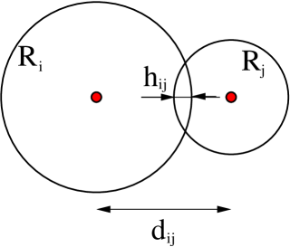
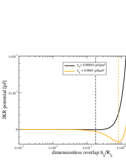
Figure 5: Illustration of the interaction model. The dynamics of two elastic and adhesive spheres in contact can be described with the JKR-potential. Left: The virtual sphere overlap $h_{ij}$ can be calculated from the sphere distance $d_{ij}=\left|\mbox{\boldmath$x$}_{i}-\mbox{\boldmath$x$}_{j}\right|$ and equilibrium radii $R_{i}$ and $R_{j}$. The circle constructed by the intersection of the sphere surfaces does not directly define the contact radius $a_{ij}$, since in real world scenarios, the spheres would evidently deform (not shown). Right: The existence of adhesive forces gives rise to bound states (right, minima at dashed lines). Their position and depth strongly depends on the parameters $\sigma_{ij}$ and $K_{ij}$. Note that the potential does not diverge at $h_{ij}/R_{ij}=2+2R_{\rm min}/R_{\rm max}$ (complete overlap). The curves on the right have been computed using the following (physiological) values $K_{ij}=1000$ Pa, $R_{ij}=2.5\rm\;\mu m$.

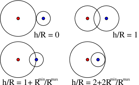
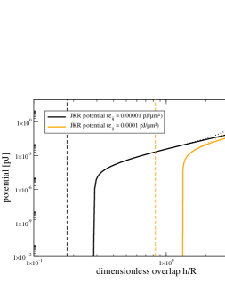
Figure 6: Sphere overlaps and modification of the interaction potential. Left: Typical contact configurations corresponding to special values of the dimensionless sphere distance $h_{ij}/R_{ij}$ – for clarity the indices have been dropped. For vanishing virtual overlap, one obtains $h/R=0$, whereas for the case when the centre of the smaller sphere is placed exactly on the boundary of the larger one, one has $h/R=1+R_{\rm min}/R_{\rm max}$. Complete inclusion of the smaller sphere within the larger one corresponds to even larger values of $h/R$. In this regime, JKR theory is not valid anymore. Right: For this reason, the JKR interaction has been supplemented with a pole at complete sphere overlap. Matching has been performed at $h_{ij}/R_{ij}=1$, where one has $\pi(\hat{\mbox{\boldmath$r$}}_{i},\hat{\mbox{\boldmath$r$}}_{j})=R_{ij}^{2}$. In the physiological regime, the potential is unchanged. Parameters have been chosen as in figure 5.

The full JKR-theory has several shortcomings:

1. It is only valid for small deformations $h_{ij}/R_{ij}\ll 1$, since the linear elastic theory assumed in the derivation of (5) is not valid for large deformations landau1959 . In addition, it approximates the cytoskeleton as a homogeneous solid, which is not the case verdier2003 . Regarding the numerical solution of the interacting particle system, this has the consequence that some cells may be completely covered by others, since the JKR force (8) does not diverge at complete overlaps. To circumvent this, a modified interaction potential has been used, which displays this divergence

   $$V(x) = f(x)V^{\rm JKR}(x)\,,$$

   $$f(x) = \left\{\begin{array}[]{ccc}\frac{(x_{\rm d}-x_{\rm m})^{2}}{(x_{\rm d}-2x_{\rm m})(x_{\rm d}-x)}-\frac{x}{x_{\rm d}-2x_{\rm m}}&:&x_{\rm m}\leq x\leq x_{\rm d}\\ 1&:&\mbox{else}\end{array}\right.\,,$$ (17)

   if one chooses as matching point $x_{\rm m}=1$ and as point for divergence $x_{\rm d}=2+2R_{\rm min}/R_{\rm max}$ (compare figure 6). The choice of this modified potential only led to significantly different growth dynamics for ${\mathcal{O}}\left(10^{4}\right)$ cells if cellular growth was constrained by static boundaries galle2005b , which indicates that the used drag forces (see appendix C) were small enough to enable fast relaxation.

2. The JKR-theory does neither include viscous effects arising from the cytoskeleton nor dissipation occurring in the extracellular matrix. Therefore, the model has been supplemented with additional drag forces, which are specified in appendix C.

3. The original result (5) has been derived as a pure two-body interaction johnson1971 , which is also the case for its purely elastic precursor hertz1882 ; landau1959 . However, for many adhering spheres already for small individual deformations additional forces will come into play, since

   • the spheres are pre-stressed,

   • the contact regions of various cells may overlap.

   Thus, the JKR model does not correctly describe cellular compression for multiple overlaps. The extent of this shortcoming will critically depend on the current adjacency topology which makes an analytical approach infeasible. For numerical ease and due to missing estimates in this article the following practitioners approach has been chosen. Below the target cell volume $V_{i/j}^{\rm target}$ the cell experiences additional repulsive – isotropic – forces due to compression of the cytoskeleton. Then, the resulting additional repulsive force acts in the direction of the neighbours $j$ with magnitude

   $$F_{ij}^{\rm comp} = A_{ij}\left[\frac{E_{i}}{3(1-2\nu_{i})}\left(1-\frac{V_{i}}{V_{i}^{\rm target}}\right)+\frac{E_{j}}{3(1-2\nu_{j})}\left(1-\frac{V_{j}}{V_{j}^{\rm target}}\right)\right]\,,$$ (18)

   where $V_{i/j}$ denote the current cellular sphere volumes (reduced by the overlaps with neighbouring spheres) and $A_{ij}$ the circular JKR contact surfaces in equation (10). Note that owing to model simplicity, neither volume nor surface corrections schaller2005a are calculated with the Voronoi tessellation in this article.

4. Whereas the forces in the approximate model (8) only depend on the actual relative cellular positions, a more realistic scenario would have to include hysteresis effects, as adhesive intercellular bonds form after contact chu2004 . This however would require to keep track of the time evolution of cellular adjacencies. In part, the time evolution can be incorporated into the time dependence of the adhesive parameters

   $$\sigma_{ij}=\frac{\sigma^{\rm max}}{2}\left[C_{i}^{\rm rec}(t)C_{j}^{\rm lig}(t)+C_{i}^{\rm lig}(t)C_{j}^{\rm rec}(t)\right]\,,$$ (19)

   where the $0\leq C_{i/j}^{\rm rec/lig}(t)\leq 1$ represent the receptor or ligand densities on the cell membrane – normalised relative to a maximum density, and $\sigma^{\rm max}$ is the maximum adhesion energy, respectively. It must be noted that also the cytoskeleton reorganises and thereby the intrinsic cell shape will not remain spherical after contact. A full description of these effects would therefore not only require time-dependent elastic parameters ($E_{i}$, $\nu_{i}$), but also the implementation of a dynamically changing intrinsic equilibrium cell-shape, which is presumably not within the reach of a centre-based model drasdo2003 ; kreft2001a .

5. In addition, the derivation of the JKR model relies on the fact that only normal forces act. For cell doublets with friction, shear forces will in reality exist. It is assumed here that the net effect of shear forces on the validity of the JKR approach can be neglected, such that they can be independently included in the drag forces.

At least for keratinocytes the application of the JKR model to cell doublet rupture experiments chu2004 leads to discrepancies between the visual equilibrium distance and the equilibrium distance predicted by the full JKR-model (5): If one derives via equation (9) the maximum adhesion energy density from the maximum rupture force recorded in chu2004 , the resulting equilibrium distance predicted by (5) is considerably different than observed in the figures of the same publication: The indentation $h_{ij}$ resulting from equation (7) becomes negative (pointing to extrapolation of JKR theory beyond the region of its validity), whereas for the approximate JKR model, the limiting condition $\sigma_{ij}/(K_{ij}R_{ij})\ll 1$ is certainly violated, which would lead to considerably smaller equilibrium distances (larger indentations) than in reality. For example, for cell-cell contact times smaller than 30 seconds, average rupture forces of 20 nN have been measured chu2004 . Assuming $K_{ij}=1000$ Pa and $R_{ij}=2.5\;\rm\mu m$ one would thereby find from equation (9) an adhesion energy density of $\sigma^{\rm max}\approx 1.7\;\rm nN/\mu m$. However, then the equilibrium distances resulting from equations (5) or (8), respectively, are inconsistent with the equilibrium distances in chu2004 . This indicates that the JKR model is not directly applicable to strongly adhesive cells. For larger times, the discrepancy becomes even worse.

However, we expect that all these shortcomings are not major sources of error if one aims at analysing control mechanisms. An improved contact model could generally be included in such simulations, but it should be reasonably motivated by microscopic theories or experimental data first.

Appendix B Random Forces

Due to thermal fluctuations, any particle in a solution will be subject to random forces (Brownian motion). In addition, some cell types exhibit intrinsic (active) movement which sometimes appear to be of random nature and thus follow the same mathematics as Brownian motion. For systems with these characteristics, the time-dependent stochastic forces $\mbox{\boldmath$F$}(t)$ modelling the random behaviour have to fulfil two conditions ma2003 :

1. their mean vanishes $\langle\mbox{\boldmath$F$}(t)\rangle=0$ and

2. the forces are not correlated, i. e., $\langle\mbox{\boldmath$F$}(t_{1})\cdot\mbox{\boldmath$F$}(t_{2})\rangle=3\xi^{2}\delta(t_{1}-t_{2})$.

The parameter $\xi$ thereby quantifies the strength of the stochastic fluctuations. The movement of single cells in a solution is highly overdamped dallon2004 , and any stochastic force fulfilling the above conditions will lead in the Langevin equation to a diffusion-like evolution of cellular distribution, i. e., in the absence of additional forces the squared displacement will be given by

$$\langle\left[\mbox{\boldmath$r$}(t)-\mbox{\boldmath$r$}_{0}\right]^{2}\rangle=3\frac{\xi^{2}}{\gamma^{2}}t=6Dt\,,$$ (20)

where $D$ is the corresponding diffusion coefficient and $\gamma$ is a dampening constant, which effectively describes the strength of friction. The above identity is also known as the fluctuation dissipation theorem, since it connects the fluctuations ($\xi$) with the dissipation ($\gamma$). If this dynamics is observed for free spherical cells in medium, the friction constant can for highly-damped dynamics be well approximated by the Stokes friction $\gamma_{0}=6\pi\eta R$, where $R$ represents the radius of the cell and $\eta$ the viscosity of the surrounding medium. Evidently, with the same random forces applied, cellular movement will be much smaller if drag forces due to cellular bindings are at work. For numerical implementations, a stochastic force fulfilling the above conditions can be given by ma2003

$$F_{i}(t) = \frac{\xi}{\sqrt{\Delta t}}\,\chi^{\rm GAUSS}_{0,1}\,,$$ (21)

where $\Delta t$ describes the width of the timestep, and $\chi^{\rm GAUSS}_{0,1}$ is a random number drawn from a Gaussian distribution matpack_manual with mean $\mu_{\chi}=0$ and width $\sigma_{\chi}=1$.

It should be noted however, that active random eucaryotic movement in reality usually occurs with pseudopods fletcher2004 : The cell attaches protrusions to neighbouring cells (or the extracellular matrix) and randomly pulls towards them. This has two further implications

• the stochastic forces become two-body forces, i. e., the neighbour cell that the pseudopod is attached to, is subject to the corresponding negative force. Also, the forces act into the direction of the normals galle2005a .

• Since the pseudopods do not enable pushing, the average stochastic force component into the direction of a given neighbour cell will not in general vanish. For example, at interfaces of dense tissue (where the pseudopods find resistance) and fluid (where no net force can be generated) one cannot expect the contributions into the different directions to compensate each other.

Since the intrinsic logic behind active cellular movement following Brownian mathematics is not fully understood and also active movement with pseudopods is not quantified for the cell types considered in the simulation (keratinocytes and melanocytes), we have chosen to implement stochastic forces via equation (21) as acting randomly on every cell that reacts passively to these in return.

Appendix C Equations of Motion

For $N$ spherical cells with positions $\mbox{\boldmath$x$}_{i}(t)$ and radii $R_{i}$ subject to cell-cell as well as cell-medium and cell-substrate interactions, the equations of motion can in the reference frame of motionless medium and boundaries be summarised as (compare also ferrez2001 )

$$m_{i}\ddot{x}_{i}^{\alpha} = F_{i}^{\alpha}+\sum_{J\in{\cal NB}(i)}F_{iJ}^{\alpha}+\sum_{j\in{\cal NN}(i)}F_{ij}^{\alpha}-\sum_{\beta}\gamma_{i}^{\alpha\beta}\dot{x}_{i}^{\beta}$$

$$-\sum_{J\in{\cal NB}(i)}\sum_{\beta}\gamma_{iJ}^{\alpha\beta}\left[\dot{x}_{i}^{\beta}+R_{i}\left(\mbox{\boldmath$n$}_{iJ}\times\mbox{\boldmath$\omega$}_{i}\right)^{\beta}\right]-\sum_{\beta}\sum_{j\in{\cal NN}(i)}\gamma_{ij}^{\alpha\beta}\left[\dot{x}_{i}^{\beta}-\dot{x}_{j}^{\beta}+R_{i}\left(\mbox{\boldmath$n$}_{ij}\times\mbox{\boldmath$\omega$}_{i}\right)^{\beta}+R_{j}\left(\mbox{\boldmath$n$}_{ij}\times\mbox{\boldmath$\omega$}_{j}\right)^{\beta}\right]\,,$$

$$I_{i}\dot{\omega}_{i}^{\alpha} = T_{i}^{\alpha}+\sum_{J\in{\cal NB}(i)}R_{i}\left(\mbox{\boldmath$n$}_{iJ}\times\mbox{\boldmath$F$}_{iJ}\right)^{\alpha}+\sum_{j\in{\cal NN}(i)}R_{i}\left(\mbox{\boldmath$n$}_{ij}\times\mbox{\boldmath$F$}_{ij}\right)^{\alpha}-\sum_{\beta}\Gamma_{i}^{\alpha\beta}\omega_{i}^{\beta}$$

$$-\sum_{J\in{\cal NB}(i)}\sum_{\beta}\Gamma_{iJ}^{\alpha\beta}\left[\dot{x}_{i}^{\beta}+R_{i}\left(\mbox{\boldmath$n$}_{iJ}\times\mbox{\boldmath$\omega$}_{i}\right)^{\beta}\right]-\sum_{\beta}\sum_{j\in{\cal NN}(i)}\Gamma_{ij}^{\alpha\beta}\left[\dot{x}_{i}^{\beta}-\dot{x}_{j}^{\beta}+R_{i}\left(\mbox{\boldmath$n$}_{ij}\times\mbox{\boldmath$\omega$}_{i}\right)^{\beta}+R_{j}\left(\mbox{\boldmath$n$}_{ij}\times\mbox{\boldmath$\omega$}_{j}\right)^{\beta}\right]\,,$$

where $\alpha,\beta\in\{0,1,2\}$ denote the Cartesian indices and $i,j\in\{0,1,\ldots,N-1\}$ the cellular indices. The first equation describes the evolution of the cell positions $\mbox{\boldmath$x$}_{i}(t)$, whereas the second equation accounts for the evolution of the cellular spin velocities $\mbox{\boldmath$\omega$}_{i}(t)$. The terming ${\cal NN}(i)$ denotes all cells having direct contact with cell $i$, whereas ${\cal NB}(i)$ refers to all boundaries in direct contact with cell $i$. Such a set of neighbouring cells can be efficiently determined as a subset of all neighbours in the weighted Delaunay triangulation of the set of spheres. (We had developed and applied such a triangulation module previously in schaller2004 ; schaller2005a .) Since for most problems few boundary conditions will be given, these are hard-wired in the code for every specific problem individually. Note that the back-reaction of the cells on the boundaries is neglected implicitly assuming that the boundaries are stationary.

The first term on the right-hand side of the first equation $F_{i}^{\alpha}$ may generally include deterministic (for example, crawling forces on a substrate) and stochastic (e. g. Brownian motion) forces on a single cell, whereas the second and third terms $\sum_{j\in{\cal NB}(i)}F_{iJ}^{\alpha}$ and $\sum_{j\in{\cal NN}(i)}F_{ij}^{\alpha}$ include the cell-boundary and intercellular two-body forces (e. g. stochastic two-body forces or the deterministic JKR-force, compare subsections B and A), respectively. The fourth term $\sum_{\beta}\gamma_{i}^{\alpha\beta}\dot{x}_{i}^{\beta}$ denotes cell-medium friction, whereas the last two terms denote dampening due to friction with the boundaries ($\gamma_{iJ}^{\alpha\beta}$) and with neighbouring cells ($\gamma_{ij}^{\alpha\beta}$), respectively. Note that the dampening forces can be divided in a contribution proportional to a relative cell velocity and a contribution arising from the angular velocities of both cells, where the normal vector $\mbox{\boldmath$n$}_{ij}$ is understood to point from cell $i$ towards cell $j$ (which restores the apparently violated antisymmetry of the dampening forces under exchange of $i$ and $j$).

The quantity $I_{i}$ on the left-hand side of the second equation denotes the inertial momentum ($I_{i}=\frac{2}{5}m_{i}R_{i}^{2}$ for rigid homogeneous spheres). In analogy with the forces, the first term on the right-hand side of the second equation $T_{i}^{\alpha}$ describes an intrinsic torque of the $i^{\rm th}$ cell, whereas the second and third terms describe the torques generated by cell-boundary and cell-cell interactions. In contrast to the forces, the dampening constant $\Gamma_{i}^{\alpha\beta}$ (capital coefficients denote rotational dampening) does not only incorporate friction with the surrounding fluid but also the dissipation of rotational energy into internal degrees of freedom of the cell (i. e., finally heat). As with the forces, the last terms describe the rotational dampening due to cell-boundary and cell-cell interaction, respectively.

Note the equation for the rotation may generally back-react onto the first equation via other channels as well. For example, the interaction forces could depend on respective angular momenta. Moreover, the terms describing the influence of the torques on the angular velocity implicitly assume that the cell is a rigid body, which is not the case. Although already sophisticated enough, the above equations should therefore be regarded a simple possible ansatz.

In the over-damped approximation

$$m_{i}\ddot{x}_{i}^{\alpha}\approx 0\qquad\mbox{and}\qquad I_{i}\dot{\omega}_{i}^{\alpha}\approx 0\,,$$ (23)

which is widely used to describe cell movements in fluids, the interaction forces and torques are always balanced by the friction forces and torques, respectively. Concerning the friction torques we assume that the internal friction of the cell is dominant ($\Gamma_{i}^{\alpha\beta}\gg\Gamma_{ij}^{\alpha\beta},\Gamma_{iJ}^{\alpha\beta}$) and that there is no intrinsic torque generated by the cell types we consider ($T_{i}^{\alpha}=0$). In addition, we assume that the dominant torque dampening is approximately isotropic ($\Gamma_{i}^{\alpha\beta}=\delta^{\alpha\beta}\Gamma_{i}$). Then, one obtains for the angular velocity

$$\Gamma_{i}\omega_{i}^{\alpha}\approx\sum_{J\in{\cal NB}(i)}R_{i}\left(\mbox{\boldmath$n$}_{iJ}\times\mbox{\boldmath$F$}_{iJ}\right)^{\alpha}+\sum_{j\in{\cal NN}(i)}R_{i}\left(\mbox{\boldmath$n$}_{ij}\times\mbox{\boldmath$F$}_{ij}\right)^{\alpha}\,.$$ (24)

If one inserts the above expression into the first equation of (C), one observes that the friction terms describing the influence of the torque on the cellular force dampening is suppressed by prefactors of $\gamma_{iJ}^{\alpha\beta}R_{i}^{2}/\Gamma_{i}$ and $\gamma_{ij}^{\alpha\beta}R_{i}^{2}/\Gamma_{i}$. Whether these terms can be neglected, is dominantly related to the structure of the cytoskeleton. We assume here that the cytoskeleton does not transmit shear forces well.

With these approximations, the relevant equations of motion take the form

$$0 \approx F_{i}^{\alpha}+\sum_{J\in{\cal NB}(i)}F_{iJ}^{\alpha}+\sum_{j\in{\cal NN}(i)}F_{ij}^{\alpha}-\sum_{\beta}\gamma_{i}^{\alpha\beta}\dot{x}_{i}^{\beta}-\sum_{J\in{\cal NB}(i)}\sum_{\beta}\gamma_{iJ}^{\alpha\beta}\dot{x}_{i}^{\beta}-\sum_{\beta}\sum_{j\in{\cal NN}(i)}\gamma_{ij}^{\alpha\beta}\left(\dot{x}_{i}^{\beta}-\dot{x}_{j}^{\beta}\right)\,.$$ (25)

Note that solving the remaining equation for the cellular spin velocities (24) is not necessary, since its back-reaction on the cell movement has been neglected and any snapshot of a rotating sphere cannot be distinguished from a motionless sphere. The above equation can be rewritten to yield

$$\sum_{k,\beta}\left\{\left[\gamma_{k}^{\alpha\beta}+\sum_{j}\gamma_{kj}^{\alpha\beta}+\sum_{J}\gamma_{kJ}^{\alpha\beta}\right]\delta_{ik}-\gamma_{ik}^{\alpha\beta}\right\}\dot{x}_{k}^{\beta}=F_{i}^{\alpha}+\sum_{j}F_{ij}^{\alpha}\,.$$ (26)

From the properties of the friction coefficients it can also be deduced that the linear system defined by this equation is symmetric and also diagonally dominant as long as $\gamma_{i}^{\alpha\alpha}+\sum_{J}\gamma_{iJ}^{\alpha\alpha}>0\qquad\forall i,\alpha$. In addition, it must be noted that the system will be extremely sparsely populated as the friction coefficients vanish for all cells not being in direct contact, see the appendix D for an example.

A usual choice for cell-medium friction is the well-known Stokes-relation $\gamma_{i}^{\alpha\beta}=6\pi\eta R_{i}\delta^{\alpha\beta}$ joos1989 introduced in subsection B. The friction coefficients and two-body forces fulfil the following conditions:

$$\gamma_{ij}^{\alpha\beta}=\gamma_{ji}^{\alpha\beta}\,,\qquad F_{ij}^{\alpha} = -F_{ji}^{\alpha}\qquad\qquad\mbox{(Newton's third axiom)}\,,$$

$$\gamma_{ij}^{\alpha\beta} = \gamma_{ij}^{\beta\alpha}\qquad\qquad\;\,\mbox{(projection operator property)}\,,$$

$$\gamma_{i}^{\alpha\beta} = \gamma_{i}\delta^{\beta\alpha}\qquad\;\;\;\;\;\;\mbox{(isotropy)}\,,$$

$$\gamma_{ii}^{\alpha\beta} = 0\qquad\qquad\;\;\;\;\;\,\mbox{(no self-friction)}\,.$$ (27)

In a strict sense, Newton’s third axiom only applies to the total two-body force. However, here the model should consistently include contact forces $F_{ij}^{\alpha}$ and drag forces $\gamma_{ij}^{\alpha\beta}\left(\dot{x}_{i}^{\beta}-\dot{x}_{j}^{\beta}\right)$, which may act independently from each other. Therefore, actio et reactio has been assumed to act separately. The symmetry in $(\alpha,\beta)$ of the friction coefficients also arises from the symmetry properties of the projection operators: The drag forces expressed by the friction coefficients may be divided in normal drag forces and tangential (shear) drag forces. Assuming that they are proportional to the effective contact area between two cells $i$ and $j$

$$A_{ij}^{\rm eff}=A_{ij}\frac{1}{2}\left[C_{i}^{\rm rec}(t)C_{j}^{\rm lig}(t)+C_{i}^{\rm lig}(t)C_{j}^{\rm rec}(t)\right]$$ (28)

and to the normal or tangential projection of the velocity differences, respectively, the friction coefficients take the form

$$\gamma_{ij}^{\alpha\beta} = A_{ij}^{\rm eff}\left(\gamma_{\parallel}{\cal P}_{ij,\parallel}^{\alpha\beta}+\gamma_{\perp}{\cal P}_{ij,\perp}^{\alpha\beta}\right)\left(1-\delta_{ij}\right)\,,$$

$$\gamma_{iJ}^{\alpha\beta} = A_{iJ}\left(\gamma_{\parallel}{\cal P}_{iJ,\parallel}^{\alpha\beta}+\gamma_{\perp}{\cal P}_{iJ,\perp}^{\alpha\beta}\right)\,.$$ (29)

The friction constant $\gamma_{\perp}$ predominantly describes internal friction within the cytoskeleton galle2005a , since force contributions for movements normal to the cell-cell contact surface are already contained within the JKR interaction model. The friction constant $\gamma_{\perp}$ is set to vanish within this article thereby implicitly assuming that dampening due to friction within the cytoskeleton is much smaller than dampening due to cell-cell bindings. In contrast, the tangential friction constant $\gamma_{\parallel}$ describes drag forces resulting from broken bindings during movements tangential to the intercellular contact plane dallon2004 ; galle2005a . For model consistency, the used contact surfaces are chosen identical with the JKR contact surface (10). Since over a wide range of physiological overlaps this relates to the spherical overlap that would result from undeformed spheres by about a factor of two, a different choice of the contact surface could be compensated by appropriately changed friction parameters.

The intercellular tangential and perpendicular projectors are given by

$${\cal P}_{ij,\parallel}^{\alpha\beta}=\delta^{\alpha\beta}-n_{ij}^{\alpha}n_{ij}^{\beta}\,,\qquad{\cal P}_{ij,\perp}^{\alpha\beta}=n_{ij}^{\alpha}n_{ij}^{\beta}\,,$$ (30)

and the cell-boundary projectors

$${\cal P}_{iJ,\parallel}^{\alpha\beta}=\delta^{\alpha\beta}-n_{iJ}^{\alpha}n_{iJ}^{\beta}\,,\qquad{\cal P}_{iJ,\perp}^{\alpha\beta}=n_{iJ}^{\alpha}n_{iJ}^{\beta}\,,$$ (31)

respectively. In the above projection operators, $\mbox{\boldmath$n$}_{ij}$ represents the normal vector pointing from cell $i$ towards cell $j$ (compare also figure 7 left panel), whereas $\mbox{\boldmath$n$}_{iJ}$ denotes the normal vector of the boundary $J$ at the contact point with cell $i$. Note that with these projection operators, the conditions on the friction coefficients (C) are automatically fulfilled.

Appendix D Numerical Solution

An example including cell-cell and cell-boundary friction is illustrated in figure 7. Indeed, for this special example all non-isotropic friction coefficients vanish except $\gamma_{03}^{\alpha\beta},\gamma_{04}^{\alpha\beta},\gamma_{23}^{\alpha\beta},\gamma_{34}^{\alpha\beta},\Gamma_{0}^{\alpha\beta},\Gamma_{4}^{\alpha\beta}$.

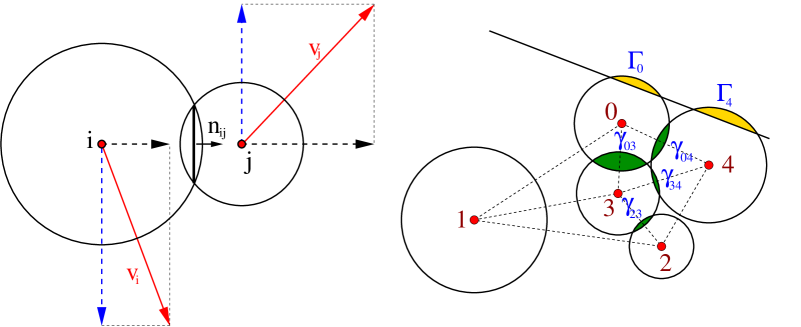
Figure 7: Two-dimensional illustration of intercellular force calculation. Left: The differential velocities between two cells $i$ and $j$ (circles) in contact may give rise to different drag forces, one proportional to the tangential part of the velocity difference and one proportional to the perpendicular part as indicated with dashed lines. Right: The dotted lines denote the weighted Delaunay triangulation of the set of spheres. Only spheres with cell-cell contact (overlap, dark grey) will contribute to intercellular friction and to intercellular forces. Cell-boundary contact (overlap, light grey) will contribute to cell-medium friction and to cell-boundary forces. Spheres that are not connected in the weighted Delaunay triangulation will not interact.

Consequently, for this example the system (26) would assume the form

$$\left(\begin{array}[]{ccccc}\mbox{\boldmath$\Gamma$}_{0}+\mbox{\boldmath$\gamma$}_{0}+\mbox{\boldmath$\gamma$}_{03}+\mbox{\boldmath$\gamma$}_{04}&{\mathbb{O}}&{\mathbb{O}}&-\mbox{\boldmath$\gamma$}_{03}&-\mbox{\boldmath$\gamma$}_{04}\\ {\mathbb{O}}&\mbox{\boldmath$\gamma$}_{1}&{\mathbb{O}}&{\mathbb{O}}&{\mathbb{O}}\\ {\mathbb{O}}&{\mathbb{O}}&\mbox{\boldmath$\gamma$}_{2}+\mbox{\boldmath$\gamma$}_{23}&-\mbox{\boldmath$\gamma$}_{23}&{\mathbb{O}}\\ -\mbox{\boldmath$\gamma$}_{03}&{\mathbb{O}}&-\mbox{\boldmath$\gamma$}_{23}&\mbox{\boldmath$\gamma$}_{3}+\mbox{\boldmath$\gamma$}_{03}+\mbox{\boldmath$\gamma$}_{34}&-\mbox{\boldmath$\gamma$}_{34}\\ -\mbox{\boldmath$\gamma$}_{04}&{\mathbb{O}}&{\mathbb{O}}&-\mbox{\boldmath$\gamma$}_{34}&\mbox{\boldmath$\gamma$}_{4}+\mbox{\boldmath$\gamma$}_{4}+\mbox{\boldmath$\gamma$}_{04}+\mbox{\boldmath$\gamma$}_{34}\end{array}\right)\left(\begin{array}[]{l}\dot{\mbox{\boldmath$x$}}_{0}\\ \dot{\mbox{\boldmath$x$}}_{1}\\ \dot{\mbox{\boldmath$x$}}_{2}\\ \dot{\mbox{\boldmath$x$}}_{3}\\ \dot{\mbox{\boldmath$x$}}_{4}\end{array}\right)=$$ (42)

$$\left(\begin{array}[]{l}\mbox{\boldmath$F$}_{0}+\mbox{\boldmath$F$}_{03}+\mbox{\boldmath$F$}_{04}+\mbox{\boldmath$F$}_{0\rm B}\\ \mbox{\boldmath$F$}_{1}\\ \mbox{\boldmath$F$}_{2}+\mbox{\boldmath$F$}_{23}\\ \mbox{\boldmath$F$}_{3}+\mbox{\boldmath$F$}_{30}+\mbox{\boldmath$F$}_{32}+\mbox{\boldmath$F$}_{34}\\ \mbox{\boldmath$F$}_{4}+\mbox{\boldmath$F$}_{40}+\mbox{\boldmath$F$}_{42}+\mbox{\boldmath$F$}_{43}+\mbox{\boldmath$F$}_{4\rm B}\\ \end{array}\right)\,,$$ (48)

where in three dimensions the symbols $\mbox{\boldmath$F$}_{i}$ and $\mbox{\boldmath$x$}_{i}$ denote vectors in ${\mathbb{R}}^{3}$ and ${\mathbb{O}}$, $\mbox{\boldmath$\gamma$}_{ij}$, $\mbox{\boldmath$\gamma$}_{i}$, and $\mbox{\boldmath$\Gamma$}_{i}$ denote $3\times 3$ matrices. This system is evidently symmetric, sparsely populated and weakly diagonally dominated, since $\gamma_{i}^{\alpha\alpha}+\Gamma_{i}^{\alpha\beta}>0\qquad\forall\qquad i,\alpha$. In addition, all friction coefficients are positive. Gershgorin’s circle theorem then suffices to guarantee positive definiteness of the dampening matrix. The number of next neighbours in contact corresponds to the number of off-diagonal blocks in the dampening matrix, such that the system becomes extremely sparse for large matrices.

Such systems can for efficiency be supplemented with the weighted Delaunay triangulation of a set of spheres for adjacency detection schaller2004 . Since the dampening matrix is positive definite, the method of conjugate gradients shewchuk1994 is well suited to the problem. However, since realistic systems will contain much more than 5 cells, the matrices would not fit into main memory, if stored completely. Fortunately, the matrices are only sparsely populated and the method of conjugate gradients can efficiently be combined with a row-indexed sparse storage scheme press1994 to compute a solution $\dot{x}_{i}^{\alpha}$. Note that the solution of the full system is an improvement over existing models: For example, in dallon2004 the tangential projector ${\cal P}_{ij}^{\alpha\beta}$ had for simplicity been approximated with the identity operator and in schaller2005a , the system was assumed to be diagonal.

The reaction-diffusion equation for the molecules

$$\frac{\partial u}{\partial t}=\nabla\left[D(\mbox{\boldmath$r$};t)\nabla u\right]+Q(\mbox{\boldmath$r$};t)$$ (50)

could in principle be solved using the method of Green functions along the lines of newman2004 . However, since spatiotemporally varying diffusion coefficients as well as nontrivial boundary conditions are considered here, the implementation of this method would require an enormous amount of work. Therefore, we have discretized above equation using the discrete element method on a cubic lattice. The arising coupled system of ordinary differential equations was then solved using the Crank-Nicolson scheme gershenfeld2000 and the algorithm of biconjugate gradients press1994 . Note that due to the strongly varying diffusion coefficients in cornified and non-cornified tissue (see table 1), the steady-state approximation is not applicable. The lattice constants for the rectangular reaction-diffusion grid discretisation have been chosen larger than the cellular diameters to ensure for validity of the discretisation approximation schaller2005a . Note that the reaction diffusion equation for the nutrients is made positive definite by cells entering necrosis below critical nutrient concentrations – necrotic cells do not consume nutrients. While the timestep of the simulation is determined by a maximum spatial cellular stepsize (fixed at $0.5\;\rm\mu m$), the timestep of the reaction-diffusion grids has been divided into several substeps such that the Courant factor press1994 is smaller than 1 in order to increase numerical accuracy. To connect the discrete reaction-diffusion grid with the spatially-continuous cellular positions, tri-linear interpolation has been used. In addition, the concentration has been fixed to vanish at grid nodes whose elementary cell did not contain cells. At grid nodes in the vicinity of cells the diffusive properties have been smoothly adapted in the range of the values given in table 1.

References

- (1) Barthel D, Matthe B, Potten CS, Owen G, Loeffler M (2000) Proliferation in murine epidermis after minor mechanical stimulation. part 2. alterations in keratinocyte cell cycle fluxes. Cell Proliferation 33:247–259.
- (2) Bashir SJ, Chew AL, Anigbogu A, Dreher F, Maibach HI (2001) Physical and physiological effects of stratum corneum tape stripping. Skin Research and Technology 7:40–48.
- (3) Bauer J, Bahmer FA, Wörl J, Neuhuber W, Schuler G, et al. (2001) A strikingly constant ratio exists between langerhans cells and other epidermal cells in human skin. A stereologic study using the optical disector method and the confocal laser scanning microscope. The Journal of Investigative Dermatology 116:313–318.
- (4) Benoit M, Gabriel D, Gerisch G, Gaub HE (2000) Discrete interactions in cell adhesion measured by single-molecule force spectroscopy. Nature Cell Biology 2:313–317.
- (5) Bettelheim E, Agam O, Shnerb NM (2001) ”Quantum phase transitions” in classical nonequilibrium processes. Physica E 9:600–608.
- (6) Brilliantov NN, Pöschel T (2004) The Physics of Granular Media, Berlin: Wiley-VCH, chapter Collision of viscoelastic particles with adhesion.
- (7) Byrne H, Preziosi L (2003) Modelling solid tumour growth using the theory of mixtures. Mathematical Medicine and Biology 20:341–366.
- (8) Carvalho G, Moore A, Qizilbash B, Lachapelle K, Schricker T (2004) Maintenance of normoglycemia during cardiac surgery. Anesthesia and Analgesia 99:319–324.
- (9) Chenevert TL, Pipe JG, Williams DM, Brunberg JA (1991) Quantitative measurement of tissue perfusion and diffusion in vivo. Magnetic Resonance in Medicine 17:197–212.
- (10) Chu YS, Thomas WA, Eder O, Pincet F, Perez E, et al. (2004) Force measurements in e-cadherin-mediated cell doublets reveal rapid adhesion strenghtened by actin cytoskeleton remodeling through rac and cdc42. Journal of Cell Biology 167:1183–1194.
- (11) Cickovski TM, Huang C, Chaturvedi R, Glimm T, Hentschel HGE, et al. (2005) A framework for three-dimensional simulation of morphogenesis. IEEE/ACM Transactions on Computational Biology and Bioinformatics 2:273–288.
- (12) Dallon J, Othmer HG (2004) How cellular movement determines the collective force generated by the dictyostelium discoideum slug. Journal of Theoretical Biology 231:203–222.
- (13) Dormann S, Deutsch A (2002) Modeling of self-organized avascular tumor growth with a hybrid cellular automaton. In Silico Biology 2:393–406.
- (14) Drasdo D, Kree R, McCaskill JS (1995) Monte carlo approach to tissue-cell populations. Physical Review E 52:6635–6657.
- (15) Drasdo D (2003) Polymer and Cell Dynamics, Basel: Birkhäuser, chapter On selected individual-based approaches to the dynamics in multicellular systems. pp. 169–204.
- (16) Edelsbrunner H, Shah N (1996) Incremental topological flipping works for regular triangulations. Algorithmica 15:223–241.
- (17) Ferreira SS, Martins ML, Vilela MJ (2002) Reaction-diffusion model for the growth of avascular tumor. Physical Review E 65:021907–021915.
- (18) Ferrez JA (2001) Dynamic triangulations for efficient 3d simulations of granular materials. Ph.D. thesis, EPFL, thesis 2432.
- (19) Fletcher DA, Theriot JA (2004) An introduction to cell motility for the physical scientist. Physical Biology 1:T1–T10.
- (20) Freyer JP, Sutherland RM (1986) Regulation of growth saturation and development of necrosis in EMT6/Ro Multicellular Spheroids by the Glucose and Oxygen Supply. Cancer Research 46:3504–3512.
- (21) Freyer JP, Sutherland RM (1986) Proliferative and clonogenic heterogeneity of cells from EMT6/Ro Multicellular Spheroids induced by the glucose and oxygen supply. Cancer Research 46:3513–3520.
- (22) Galle J, Loeffler M, Drasdo D (2005) Modeling the effect of deregulated proliferation and apoptosis on the growth dynamics of epithelial cell populations in vitro. Biophysical Journal 88:62–75.
- (23) Galle J, Aust G, Schaller G, Beyer T, Drasdo D (2006) Individual Cell-Based Models of the Spatial-Temporal Organisation of Multicellular Systems – Achievements and Limitations. Cytometry 69A:704–710.
- (24) Gammel BM (2003) Matpack C Numerics and Graphics Library 1.7.3. .
- (25) Gardner M (1970) Mathematical games. Scientific American :120–123.
- (26) Gatenby RA, Maini PK (2003) Cancer summed up. Nature 421:321–322.
- (27) Gershenfeld N (2000) The Nature of Mathematical Modeling. Cambridge: Cambridge University Press.
- (28) Graner F, Glazier JA (1992) Simulation of biological cell sorting using a two-dimensional extended potts model. Physical Review Letters 69:2013–2016.
- (29) Hertz H (1882) Über die Berührung fester elastischer Körper. Journal für die reine und angewandte Mathematik 92:156–171.
- (30) Hoath SB, Leahy DG (2003) The organization of human epidermis: Functional epidermal units and phi proportionality. The Journal of Investigative Dermatology 121:1440–1446.
- (31) Johnson KL (1958) A note on the adhesion of elastic solids. British Journal of Applied Physics 9:199–200.
- (32) Johnson KL, Kendall K, Roberts AD (1971) Surface energy and the contact of elastic solids. Proceedings of the Royal Society of London A 324:301–313.
- (33) Joos G (1989) Lehrbuch der Theoretischen Physik. Wiesbaden: AULA-Verlag, edition.
- (34) Kasting GB, Barai ND, Wang TF, Nitsche JM (2003) Mobility of water in human stratum corneum. Journal of Pharmaceutical Sciences 92:2326–2340.
- (35) Kreft JU, Booth G, Wimpenny JWT (1998) Bacsim, a simulator for individual-based modelling of bacterial colony growth. Microbiology 144:3275–3287.
- (36) Kreft JU, Picioreanu C, Wimpenny JWP, van Loosdrecht MCM (2001) Individual-based modelling of biofilms. Microbiology 147:2897–2912.
- (37) Kreft JU (2004) Biofilms promote altruism. Microbiology 150:2751–2760.
- (38) Landau LD, Lifshitz EM (1959) Theory of Elasticity. London: Pergamon Press.
- (39) Livingston EH, Engel E (1995) Modeling of the gastric gel mucus layer: application to the measured ph gradient. Journal of Clinical Gastroenterology 21:S120–S124. Suppl. 1.
- (40) Louzoun Y, Solomon S, Atlan H, Cohen IR (2003) Proliferation and competition in discrete biological systems. Bulletin of Mathematical Biology 65:375–396.
- (41) Ma Q, Izaguirre JA (2003) Long time step molecular dynamics using targeted Langevin stabilization. In: Proceedings of the 2003 ACM symposium on Applied computing. Symposium on Applied Computing, New York, NY, USA: ACM Press, pp. 178–182.
- (42) Mahaffy RE, Shih CK, MacKintosh FC, Käs J (2000) Scanning probe-based frequency-dependent microrheology of polymer gels and biological cells. Physical Review Letters 85:880–883.
- (43) Maniotis AJ, Chen CS, Ingber DE (1997) Demonstration of mechanical connections between integrins, cytoskeletal filaments, and nucleoplasm that stabilize nuclear structure. Proceedings of the National Academy of Sciences USA 94:849–854.
- (44) Meineke F, Potten C, Loeffler M (2001) Cell migration and organization in the intestinal crypt using a lattice-free model. Cell Proliferation 34:253–266.
- (45) Meyer-Hermann M, Maini PK (2004) Interpreting two-photon imaging data of lymphocyte motility. Pysical Review E 71:061912.
- (46) Moncrieff M (2001) The clinical application of spectrophotometric intracutaneous analysis for the diagnosis of cutaneous malignant melanoma. Ph.D. thesis, University of East Anglia.
- (47) Montagna W, Kligman AM, Charlisle KS (1992) Atlas of Normal Human Skin. New York: Springer Verlag.
- (48) Moy VT, Jiao Y, Hillmann T, Lehmann H, Sano T (1999) Adhesion Energy of Receptor-Mediated Interaction Measured by Elastic Deformation. Biophysical Journal 76:1632–1638.
- (49) Murray JD (2002) Mathematical Biology I, volume 17 of Interdisciplinary Applied Mathematics. Berlin Heidelberg: Springer, edition.
- (50) von Neumann J (1966) Theory of Self-Reproducing Automata. University of Illinois Press, edition.
- (51) Newman TJ, Grima L (2004) Many-body theory of chemotactic cell-cell interactions. Physical Review E 70:051916.
- (52) Norlen L, Al-Amoudi A (2004) Stratum corneum keratin structure, function, and formation: The cubic rod-packing and membrane templating model. The Journal of Investigative Dermatology 123:715–732.
- (53) Picioreanu C, Kreft JU, van Loosdrecht MCM (2004) Particle-based multidimensional multispecies biofilm model. Applied and Environmental Microbiology 70:3024–3040.
- (54) Potten CS, Li YQ, Ohlrich R, Matthe B, Loeffler M (2000) Proliferation in murine epidermis after minor mechanical stimulation. part 1. sustained increase in keratinocyte production and migration. Cell Proliferation 33:231–246.
- (55) Press WH, Teukolsky SA, Vetterling WT, Flannery BP (1994) Numerical Recipes in C. Cambridge University Press, edition.
- (56) Savill NJ, Sherratt JA (2003) Control of epidermal stem cell clusters by notch-mediated lateral induction. Developmental Biology 258:141–153.
- (57) Schaller G, Meyer-Hermann M (2004) Kinetic and dynamic delaunay tetrahedralizations in three dimensions. Computer Physics Communications 162:9–23.
- (58) Schaller G, Meyer-Hermann M (2005) Multicellular tumor spheroid in an off-lattice Voronoi/Delaunay cell model. Physical Review E 71:051910–16.
- (59) Schaller G, Meyer-Hermann M (2006) Continuum versus Discrete model: A comparison for multicellular tumour spheroids. Philosophical Transactions of the Royal Society Series A 364:1443–1464.
- (60) Schwindt DA, Wilhelm KP, Maibach HI (1998) Water diffusion characteristics of human stratum corneum at different anatomical sites in vivo. The Journal of Investigative Dermatology 111:385–389.
- (61) Shewchuk JR (1994) An introduction to the conjugate gradient method without the agonizing pain. Technical report, Carnegie Mellon University, Pittsburgh, PA, USA.
- (62) Smolle J (1998) Cellular automaton simulation of tumour growth – equivocal relationships between simulation parameters and morphologic pattern features. Analytical Cellular Pathology 17:71–82.
- (63) Tang A, Eller MS, Hara M, Yaar M, Hirohashi S, et al. (1994) E-cadherin is the major mediator of human melanocyte adhesion to keratinocytes in vitro. Journal of Cell Science 107:983–992.
- (64) Tuchin VV, Bashkatov AN, Genina EA, Sinichkin YP, Lakodina NA (2001) In vivo investigation of the immersion-liquid-induced human skin clearing dynamics. Technical Physics Letters 27:489–490.
- (65) Turner S, Sherratt JA (2002) Intercellular Adhesion and Cancer Invasion: A Discrete Simulation Using the Extended Potts Model. Journal of Theoretical Biology 216:85–100.
- (66) Verdier C (2003) Rheological properties of living materials. from cells to tissues. Journal of Theoretical Medicine 5:67–91.
- (67) Wehrle JP, Ng CE, McGovern KA, Aiken NR, Shungu DC, et al. (2000) Metabolism of alternative substrates and the bioenergetic status of EMT6 tumor cell spheroids. NMR in Biomedicine 13:349–460.
- (68) Weliky M, Oster G (1990) The mechanical basis of cell rearrangement. Development 109:373–386.
- (69) Weliky M, Oster G, Minsuk S, Keller R (1991) Notochord morphogenesis in xenopus laevis: Simulation of cell behavior underlying tissue convergence and extension. Development 113:1231–1244.