Income Distribution Dependence of Poverty Measure: A Theoretical Analysis

Abstract

With a new deprivation (or poverty) function, in this paper, we theoretically study the changes in poverty with respect to the ‘global’ mean and variance of the income distribution using Indian survey data. We show that when the income obeys a log-normal distribution, a rising mean income generally indicates a reduction in poverty while an increase in the variance of the income distribution increases poverty. This altruistic view for a developing economy, however, is not tenable anymore once the poverty index is found to follow a pareto distribution. Here although a rising mean income indicates a reduction in poverty, due to the presence of an inflexion point in the poverty function, there is a critical value of the variance below which poverty decreases with increasing variance while beyond this value, poverty undergoes a steep increase followed by a decrease with respect to higher variance. Following these results, we make quantitative predictions to correlate a developing with a developed economy.

JEL classification number: I32, D63

Key words: Poverty; Inequality; Income distribution; Consumption deprivation; Inflexion point.

1 Introduction

Since the paradigmatic contribution of Sen [15, 17] and Atkinson [1], a remarkable amount of effort has been undertaken [7, 9] in theoretically understanding the economics of poverty and inequality. The studies range from being aptly mathematical in nature to a qualitative characterisation of such population dialectics. Pradhan and Ravallion [13] have used qualitative assessments of perceived consumption adequacy based on a household survey. They claim that perceived consumption needs can be a more promising approach than the subjective income-based poverty line. This consumption norm can correspond to a saturation level of consumption, below which the individual could be considered to be in poverty. Further, in this paper, our approach is rather complementary to a lemma-based mathematical model in that we use survey based consumption data to quantify the dependence of a well-known poverty function [6, 8] on the mean and variance of the income distribution. To this end, we use income-expenditure data from a ‘developing nation’ (India in our case) and utilise the well established technique of data fitting to define the per capita consumption as a function of income. Here the implicit assumption is that of a near equilibrium situation such that the time dependence of both income and consumption variables can be considered as transients without much effect on the asymptotic distributions. Deaton [5] has discussed the ambiguity that arises using survey data versus national accounts data for individual consumption or income levels. Although the survey consumption data seem to understate the true consumption levels, we are however using the data as a backup to our analytical results thereby restricting our claims to being qualitative in nature. Such comparisons with real data help us have approximate ideas of the values of the unknown parameters, two in our model, although the general conclusions are remarkably independent of these parameter values.

Assuming that the income distribution can be characterised by a two-parameter function, such as a log-normal distribution, in the first section of the paper we study the effects of changes in the mean and variance of the underlying income distribution on poverty. The results of this analysis indicate that an increase in mean income and a reduction in the variance of income distribution can reduce poverty. It also hints towards a trade-off, in that while an increase in average income reduces poverty, a simultaneous increase in income variance can escalate poverty. This result is likely to suggest that reducing income inequality should be the precondition for lowering poverty. These general results are then contrasted in the following section using a different model for the income distribution, the pareto distribution. The objective is basically to probe whether the results obtained are universal in nature and if not, then which distribution defines a better measure of poverty.

2 Poverty impact of changes in log-normal income distribution

Poverty equals consumption deprivation on an essential food. The necessity of defining poverty as a multidimensional concept rather than relying on income or consumption expenditures per capita has been well documented. Although it is important to assess deprivation with more than one attribute (see [2, 3, 6, 12]), we consider the case of most essential food item that is required for survival, in an attempt to include deprivation into the poverty index. Such an index would suggest that a person can be considered poor if the individual’s consumption falls within the deprivation area in the diagram (see lower panel of Fig.1), that is, the cumulative difference between the saturation consumption level of cereal and actual cereal consumption by the community as a whole. The upper panel of Fig.1 shows positive consumption even at zero income level, which makes our formulation more realistic than the non-linear function used in Kumar et al. [10]. The non-linear function used in our paper that allows a saturation level of consumption norm for food-grains is as follows:

$$C(y)=\frac{V\exp(y)}{K+\exp(y)}$$ (1)

where $C$ is the consumption expenditure on food-grains, $y$ is income and the parameters $V,\>\>K(>0)$ represent the saturation level of real food-grain consumption expenditure or the bliss level and the level of income needed to consume one half of the saturation level respectively. Consumption deprivation (CD) or poverty (P) can be defined as the shortfall of actual consumption expenditure relative to saturation level V, or $CD=V-C$. Thus the non-linear CD function is derived as:

$$CD=\frac{VK}{K+\exp(y)}$$ (2)

This function, being a convex decreasing function of income provides a direct measure of poverty based on nutritional norms, while $V$ and $K$ are parameters of a concave Engel curve. Here $C\rightarrow V$ represents the idealistic limit where there is no deprivation or poverty corresponding to a static equilibrium in the social dialectics mathematically represented by $y=y^{*}$. In what follows, we would consider two asymptotic regimes - $y\rightarrow 0$ and $y\rightarrow\infty$ - physically which correspond to the low and high income groups respectively. Naturally our focus would be on the $y\rightarrow 0$ limit, that is on the low income section although the analysis would encompass both limits.

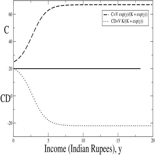
Figure 1: Consumption C(y) and deprivation CD(y) functions against income y

If consumption of the most essential food item follows a concave non-linear functional form and if individual poverty is measured as the difference between the saturation level of consumption of the essential food item and its actual level, assumption of a log-normal income distribution implies a reduction in poverty with the increase of mean income of the population and an increase in inequality with increasing poverty. This new measure of poverty is based on the notion of consumption deprivation of a very essential staple food such as rice or wheat (cereal), derived from a nonlinear, monotonically increasing concave consumption function varying with the income, albeit with no specific reference to a subjective poverty line. The standard log-normal probability density function (pdf) is defined as

$${\rm f}(y/\mu,\sigma^{2})=\frac{1}{y\sigma\sqrt{2\pi}}\>\exp[-\frac{{(lny-\mu)}^{2}}{2{\sigma}^{2}}]$$ (3)

where y is normally distributed with mean $\mu$ and variance $\sigma^{2}$ (both positive real numbers). With this log-normal pdf for the income y, the poverty equation can be rewritten as follows:

$$P = \int_{0}^{\infty}\>CD(y)\>{\rm f}(y)dy$$ (4)

$$= \int_{0}^{\infty}\>\frac{VK}{K+\exp(y)}\>\frac{1}{y\sigma\sqrt{2\pi}}\>\exp[-\frac{{(lny-\mu)}^{2}}{2{\sigma}^{2}}]\>dy$$

Partial derivatives of the above equation (4) with respect to $\mu$ and $\sigma^{2}$ give

$$\frac{\partial P}{\partial\mu} = \int_{0}^{\infty}\>\frac{VK}{K+\exp(y)}\>\frac{1}{y\sigma\sqrt{2\pi}}$$

$$\times \exp[-\frac{{(lny-\mu)}^{2}}{2{\sigma}^{2}}]\frac{lny-\mu}{\sigma^{2}}\>dy$$

$$\frac{\partial P}{\partial{\sigma^{2}}} = \int_{0}^{\infty}\>\frac{VK}{K+\exp(y)}\>\frac{1}{2y{\sigma^{3}}\sqrt{2\pi}}$$ (5)

$$\times \exp[-\frac{{(lny-\mu)}^{2}}{2{\sigma}^{2}}]\>[\frac{{(lny-\mu)}^{2}}{\sigma^{2}}-1]\>dy$$

P satisfies the three standard axioms of a poverty index , namely the monotonicity, transfer, and transfer sensitivity axioms that any such index must satisfy.

2.1 Asymptotic solutions of the poverty function

This section deals with asymptotic solutions of the poverty functions for extremely low ($y\rightarrow 0$) to moderate values of the income distribution. This is mathematically categorised in the following manner:

For moderate incomes, $C(y)=\frac{V\exp(y)}{K+\exp(y)}=C_{{\rm mod}}(y)$, say,

1. $C_{{\rm mod}}(y\rightarrow 0)=\frac{V}{K+1}$ $\&$
2. $C_{{\rm mod}}(y\rightarrow\infty)=V$

whereas for very low income groups, $C(y)=\frac{Vy}{K+y}=C_{{\rm\ low}}(y)$, say,

1. $C_{{\rm low}}(y\rightarrow 0)=0$ $\&$
2. $C_{{\rm low}}(y\rightarrow\infty)=V$

The above comparison clearly shows that although both definitions of the consumption function are generally equivalent in the low income limit, for the absolutely needy groups, $C_{{\rm mod}}(y)$ predicts a non-zero ($\frac{V}{K+1}$) lower limit of income which is more realistic than $C_{{\rm low}}(y\rightarrow 0)=0$. A linear stability analysis of $C_{{\rm low}}(y)$ also shows that $y=0$ is an unstable fixed point, which further strengthens this conviction. Henceforth our attention will mainly be focused towards the lowest income groups defined by $C_{{\rm low}}(y)$, although we would flip back and forth between the moderate to the low income classes for comparisons. Before proceeding any further, though, we first derive the values of the parameters $V,K$ by fitting the function $C_{{\rm mod}}$ with actual survey data obtained from National Sample Survey, 1999-2000, 55th Round, India. We would be using these values of $V,K$ in all analyses in this paper. Fig.2 portrays the shape of an Engle curve, graphing real cereal expenditure against the total expenditure - a surrogate for income.

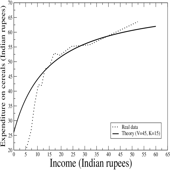
Figure 2: Consumption C(y) plotted against income y: data fitting to evaluate V and K using data from Indian National Sample survey 1999-2000, 55^th round.

The above exact data fitting conclusively shows that the parameters $V$ and $K$ have the respective values 45 and 15 in Indian currency (Rupees). These are roughly equivalent to 1.0 USD and 0.33 USD respectively. Now using these values, we study the case for typically the lowest income classes defined by the consumption function $C_{{\rm low}}(y)$. In this case, however, we need to focus on both low and high limits of the variance. Upto first order in $\sigma^{2}$, we find that

$${P_{{\rm low}}}_{\sigma\rightarrow 0}=\frac{V}{K}[K-\exp(-{\mu-\frac{\sigma^{2}}{2}})]$$ (6)

The poverty dependence on the mean for this asymptotic regime can be understood from figure 3.

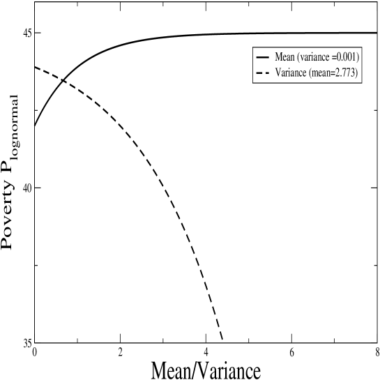
Figure 3: Poverty versus mean $\mu$ (for fixed variance $\sigma^{2}=0.001$) and versus variance $\sigma^{2}$ (for a fixed mean $\mu=2.773$) for a log-normal distribution for the limiting case $\sigma^{2}\rightarrow 0$ defined by equation (6).

Fig. 3 tells us that poverty is a monotonically decreasing function of variance for a fixed mean (taken to be 2.773 for a direct comparison with Fig. 4 later). On the other hand, for a fixed variance (0.001), poverty increases with mean and then saturates after a critical value. This result is very remarkable but needs to be taken with a pinch of salt, especially since this is true only in the asymptotic ($\sigma\rightarrow 0$) regime. We will revisit this problem in the following section where we discuss the situation when both the mean and the variance of the income distribution are simultaneously varying.

2.2 Overall impact of simultaneous changes in mean and variance

Here we show what effect any change, either increase or decrease, in the income distribution has on the overall poverty function when the distribution is log-normal and when both mean and variance are varying. Since our focus is on the low income group, we will be using $C_{{\rm low}}(y)$ as our definition for the consumption function. The attention here would be to decipher the joint variation of the poverty function $P(\mu,\sigma^{2})$ with respect to $\mu$ and $\sigma^{2}$. Once again using a $1/y$ expansion upto the first order, we find that the joint poverty function reads as

$$dP(\mu,\sigma^{2}) = \frac{\partial P}{\partial\mu}d{\mu}+\frac{\partial P}{\partial{\sigma^{2}}}d{\sigma^{2}}$$ (7)

$$= \frac{VK}{\sigma^{2}}\exp[-(\mu-\frac{\sigma^{2}}{2})]\>d{\mu}$$

$$+ \frac{VK}{2}\exp[-(\mu-\frac{\sigma^{2}}{2})A]\>d{\sigma^{2}}$$

This equation suggests that poverty is a decreasing function of changes in $\mu$ and an increasing function of changes in $\sigma$². For a fixed variance, d$\sigma$²=0, and hence the first component of [7], reflecting change in $\mu$, will provide convergence; and with a fixed mean, d$\mu$=0, the second component, exhibiting change in $\sigma$², will give convergence of the equation. When both the mean and variance of the income distribution change as a result of changes in macroeconomic policies, their effect on poverty can be evaluated via equation (7). The notable point here is the fundamental qualitative difference with the prediction from equation (6). As opposed to the earlier asymptotic result where increase of the mean income was expected to generate a positive augmentation in poverty (for fixed variance) followed by a saturation at a particular value $\mu_{c}$, equation (7) with a fixed $\sigma$ clearly suggests that poverty decreases with increase of the mean income. This apparent dichotomy can be understood once we analyse the physical meaning hidden in equation (6). It says that in a relatively large group of low earning population, a very small variance between the earners contributes to an increase in poverty for very low to moderate values of the mean income. However, once the mean income reaches a critical value, this spurious effect saturates off. This can be contrasted with the prediction from the last equation which holds true for moderate to large values of $\sigma$. We would like to specifically point out here that both predictions from equations (6, 7) are true but in their respective regimes defined by small to large values of $\sigma$.

3 Poverty impact of changes in pareto income distribution

In this section, our objective is to study the mean and variance dependence of the poverty function, replacing the log-normal probability distribution, previously assumed, with a pareto distribution and contrast the findings later. Once again we would conform to the same consumption and deprivation functions (1,2) and try to understand the qualitative changes in the poverty function of a growing economy with respect to changes in the mean and variance of the overall income distribution.

The standard pareto probability density function $f_{{\rm pareto}}$ defined over the interval $y\geq b$ is given by

$${\rm f}_{{\rm pareto}}(y)=\frac{ab^{a}}{y^{a+1}}$$ (8)

where the mean $\mu$ and the variance $\sigma^{2}$ can be easily shown to be as follows

$$\mu = \frac{ab}{a-1}$$

$$\sigma^{2} = \frac{ab^{2}}{{(a-1)}^{2}(a-2)}$$ (9)

With this pareto probability density function, the poverty function $P_{{\rm pareto}}$ reads as follows

$$P_{{\rm pareto}}(a,b) = \int_{0}^{\infty}\>CD(y){\rm f}_{{\rm pareto}}(y)dy$$ (10)

$$= VKab^{a}\>\int_{b}^{\infty}\>\frac{dy}{(K+y)y^{a+1}}$$

$$= \frac{V}{K}\>[1-ab^{a}\int_{b}^{\infty}\>dy\frac{1}{(K+y)y^{a}}]$$

Defining the identity $I(a)=\int_{b}^{\infty}\>\frac{dy}{(K+y)y^{a+1}}$, and taking recourse to a bit of algebra one can deduce a recursive relation

$$I(a) = \frac{1}{Kab^{a}}[1-\frac{ab}{K(a-1)}+\frac{ab^{2}}{K^{2}(a-2)}]$$ (11)

$$- \frac{1}{K^{3}}I(a-3,b)$$

This equation (11) can be correlated with a hypergeometric ${}_{2}F_{1}$ series and for specified values of the parameters can be solved numerically. For our purpose though, we consider the limit $a\rightarrow\infty$ to have a first hand impression of the situation

$$P(a\rightarrow\infty,b)=\frac{V}{K}\>[1-\frac{1}{K}\frac{1}{1+\frac{b}{K}}]$$ (12)

We would now directly evaluate the poverty function in a more physical limit. Without any loss of generality we choose the limit $K\rightarrow 0$ which is akin to the 1/y expansion we did in deriving the poverty function for the log-normal distribution. We would shortly see that in this case, this basic expansion allows us to have an ‘exact’ derivation of the poverty function as opposed to its log-normal counterpart. Upto the first order in 1/y and utilising equation (9), we find

$$P(a,b)=VK[\frac{1}{\mu}\frac{a^{2}}{a^{2}-1}-\frac{1}{\mu^{2}}\frac{a^{3}}{{\ (a-1)}^{2}(a+2)}]$$ (13)

where $a=2+\sqrt{1+\frac{\mu^{2}}{\sigma^{2}}}$ and $b=\frac{a-1}{a}\mu$. A numerical solution of the above equation (13) shows that it has a pair of inflexion points , out of which the physical pair is at $\mu=3.05139\>\>\&\>\>\sigma^{2}=0.0692138$. Solving around this inflexion point, we now come across one of the most remarkable results of this article, the fact that poverty initially decreases with increasing variance until it reaches a critical value $\sigma^{2}={\sigma_{c}}^{2}$ beyond which the poverty starts increasing with variance followed by a dip once again.

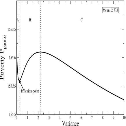
Figure 4: Poverty versus mean $\mu$ for fixed variance in a pareto distribution close to the inflexion point($\mu=2.773$). Zone A represents an under-developed economy; zone B defines the poverty- variance relation for a developing nation; zone C represents an economically developed nation.

Fig. 4 has been drawn using $\sigma^{2}=2.773$, a value reasonably close to the inflexion point. The plot shows that poverty decreases until it reaches the point $\mu_{c}\sim 0.25$ after which it starts increasing approximately until $\sigma^{2}=2$ and then it starts decreasing again. This result is in marked contrast with the log-normal case where the poverty rather uninterestingly decreases with increasing mean for a fixed variance, and increases with for a fixed mean. It is now not difficult to pinpoint the detailed meaning of this result. Referring to Fig. 4, zone A defines a rather ‘underdeveloped’ economy, zone B stands for a ‘developing’ economy, our case in study, while the final zone C clearly indicates what one would expect in the case of an economically ‘developed’ nation. We can probably claim without much ambiguities that a pareto distribution has the power to encapsulate all three modes of economies and is the ideal candidate for all future studies involving poverty measure. Further, zones B and C appear to suggest an inverted-U hypothesis similar to Kuznets [11] that poverty increases in the early stages of development and subsequently it declines with higher level of economic progress even though such development is associated with higher inequality.

4 Conclusion

This paper made use of a poverty function, which is different from the conventional poverty indices in the following manner: (1) the CD index does not depend on an arbitrarily chosen poverty line, (2) it depends on the observed and measurable consumption behaviour of people, (3) the index satisfies the standard axioms of a poverty index. Having used such a consumption deprivation function as a measure of poverty, this paper has shown analytically that for a log-normal income distribution, an increase in mean income, ceteris paribus, will decrease poverty while an increase in the variance of the income distribution, ceteris paribus, will increase poverty although somewhat contradictory information was obtained for the limiting case of earners with extremely low variance in their income distribution. In this case, poverty was found to decrease with increasing variance for a fixed mean, while when plotted against the mean (Fig. 3), it was found to initially increase and then saturate after a critical value of the mean which we could determine theoretically.

These observations were later contrasted with observations made from a pareto distribution. Here we found that for very low earning groups in a developing economy, poverty initially decreases with increasing variance but beyond a critical value of the variance, it starts increasing later to decrease again. In the process, this defines all three economies characterised by individual parametric regimes. The conclusion that we derive from these joint analyses is that the variance dependence of poverty is not unequivocally simplistic, in that one distribution (log-normal) predicts an increase in poverty with increasing variance (although the limiting $\sigma^{2}\rightarrow 0$ case was somewhat qualitatively identical to zone B for the pareto distribution) while the other (pareto) shows the existence of an inflexion point in the poverty function. This means that the poverty-variance graph in a pareto distribution has a critical point, on one side (zone A) of which poverty decreases with increasing variance, while on the other side it is just the reverse.

Our contribution here is to prove that a pareto distribution offers the more realistic measure of poverty in a developing economy. This is because it condones the very realistic fact that for very low income groups a slight increase in the variance only serves to decrease poverty whereas for high earning groups, greater the variation in earning greater is the probability of an escalation in poverty up to another critical point, beyond which poverty declines with any further increase in variance of wealth distribution in a society. This phase seems to reflect the case of a very developed economy, one which we identify as the supra-economic behaviour. In macroeconomic sense, this phase suggests that close to an equilibrium dynamics, higher inequality could contribute to higher savings and thereby higher growth and reduced poverty. In a follow-up work [4], shortly to be communicated, we have shown that in the non-stationary case, where both income and consumption are functions of time, the consumption deprivation dynamics can be mapped to the paradigmatic Burgers’ equation, thereby bestowing us with the ability to make quantitative predictions on the poverty of a developing economy as a function of income and time.

References

- [1] Atkinson, A. B., 1987, On the Measurement of Poverty, Econometrica, 55 (4): 749-764.
- [2] Atkinson, A.B., 2003, Multidimensional Deprivation: Contrasting Social Welfare and Counting Approaches, The Journal of Economic Inequality, 1 (1): 51-65.
- [3] Bourguignon, F., and S.R. Chakravarty, 2003, The Measurement of Multidimensional Poverty, The Journal of Economic Inequality, 1 (1): 25-49.
- [4] Chattopadhyay, A. K. and Mallick, S. K., A Stochastic Measure of Poverty, unpublished.
- [5] Deaton, A., 2005, Measuring Poverty in a Growing World (or Measuring Growth in a Poor World), The Review of Economics and Statistics, 87 (1): 1-19.
- [6] Dutta, I., P.K. Pattanaik, and Y. Xu, 2003, On Measuring Deprivation and the Standard of Living in a Multidimensional Framework on the Basis of Aggregate Data, Economica, 70 (278): 197-221.
- [7] Foster, J.E., J. Greer and E. Thorbecke, 1984, A class of decomposable poverty measures, Econometrica, 52: 761-766.
- [8] Foster, J.E. and A.F. Shorrocks, 1991, Subgroup consistent poverty indices, Econometrica, 59: 667 709.
- [9] Kakwani, N.C., 1980, On a class of poverty measures, Econometrica, 43: 437-446.
- [10] Kumar, T.K., Gore, A.P., and Sitaramam, V., 1996, Some Conceptual and Statistical Issues on Measurement of Poverty, Journal of Statistical Planning and Inference, Econometric Methodology, Part I, 49 (1): 53-71.
- [11] Kuznets, S., 1955, Economic Growth and Income Inequality, The American Economic Review, 45 (1): 1–28.
- [12] Mukherjee, D., 2001, Measuring multidimensional deprivation, Mathematical Social Sciences, 42 (3): 233-251.
- [13] Pradhan, M. and M. Ravallion, 2000, Measuring Poverty Using Qualitative Perceptions of Consumption Adequacy, The Review of Economics and Statistics, 82 (3): 462-471.
- [14] Rao, V.V.B., 1981, Measurement of deprivation and poverty based on the proportion spent on food: An exploratory exercise, World Development, 9 (4), April, 337-353.
- [15] Sen, A. K., 1973, On Economic Inequality, Oxford: Clarendon Press.
- [16] Sen, A.K., 1976, Poverty: An Ordinal Approach to Measurement, Econometrica, 44: 219–231.
- [17] Sen, A. K., 1979, Issues in the Measurement of Poverty, Scandinavian Journal of Economics 8: 285-307.