Geometrical aspects of first-order optical systems

Abstract

We reconsider the basic properties of ray-transfer matrices for first-order optical systems from a geometrical viewpoint. In the paraxial regime of scalar wave optics, there is a wide family of beams for which the action of a ray-transfer matrix can be fully represented as a bilinear transformation on the upper complex half-plane, which is the hyperbolic plane. Alternatively, this action can be also viewed in the unit disc. In both cases, we use a simple trace criterion that arranges all first-order systems in three classes with a clear geometrical meaning: they represent rotations, translations, or parallel displacements. We analyze in detail the relevant example of an optical resonator.

Keywords: Geometrical methods, matrix methods, paraxial optical systems, optical resonators.

1 Introduction

Matrix methods [1, 2] offer the great advantage of simplifying the presentation of linear models and clarifying the common features and interconnections of distinct branches of physics [3]. Modern optics is not an exception and a wealth of input-output relations can be compactly expressed by a single matrix [4]. For example, the well-known $2\times 2$ ray-transfer matrix, which belongs to the realm of paraxial ray optics, predicts with almost perfect accuracy the behavior of a Gaussian beam.

In this respect, we note that there is a wide family of beams (including Gaussian Schell-model fields, which have received particular attention [5, 6, 7, 8, 9, 10, 11, 12, 13, 14, 15]) for which a complex parameter can be defined such that, under the action of first-order systems, it is transformed according to the famous Kogelnik $ABCD$ law [16, 17, 18, 19, 20]. This is the reason why they are so easy to handle. This simplicity, together with the practical importance that these beams have for laser systems, explain the abundant literature on this topic [21, 22].

The algebraic basis for understanding the transformation properties of such beams is twofold: the ray-transfer matrix of any first-order system is an element of the group SL(2, $\mathbb{R}$) [23] and the complex beam parameter changes according to a bilinear (or Möbius) transformation [24].

The nature of these results seems to call for a geometrical interpretation. The interaction between physics and geometry has a long and fruitful story, a unique example is Einstein theory of relativity. The goal of this paper is precisely to provide such a geometrical basis, which should be relevant to properly approach this subject.

The material of this paper is organized as follows. In section 2 we include a brief review of the transformation properties of Gaussian beams by first-order systems, introducing a complex parameter $Q$ to describe the different states as points of the hyperbolic plane. The action of the system in terms of $Q$ is then given by a bilinear transformation, which is characterized through the points that it leaves invariant. From this viewpoint the three basic isometries of this hyperbolic plane (i.e., transformations that preserve the distance), namely, rotations, translations, and parallel displacements, appear linked to the fact that the trace of the ray-transfer matrix has a magnitude lesser than, greater than, or equal to 2, respectively.

In section 3 we present a mapping that transforms the hyperbolic plane into the unit disc (which is the Poincaré model of the hyperbolic geometry) and we proceed to study the corresponding motions in this disc. Finally, as a direct application, in section 4 we treat the case of periodic systems, which are the basis for optical resonators, providing an alternative explanation of the standard stability condition.

We emphasize that this geometrical scenario does not offer any advantage in terms of computational efficiency. Apart from its undeniable beauty, its benefit lies in gaining insights into the qualitative behaviour of the beam evolution.

2 First-order systems as transformations in the hyperbolic plane $\mathbb{H}$

We consider the paraxial propagation of light through axially symmetric systems, containing no tilted or misaligned elements. The reader interested in further details should consult the extensive work of Simon and Mukunda [25, 26, 27, 28, 29]. We take a Cartesian coordinate system whose $Z$ axis is along the axis of the optical system and represent a ray at a plane $z$ by the transverse position vector $x(z)$ (which can be chosen in the meridional plane) and by the momentum $p(z)=n(z)dx/dz$ [30]. Here $n(z)$ is the refractive index and $dx/dz$ is the direction of the ray through $z$.

At the level of ray optics, a first-order system changes the ray parameters by the simple transformation [31]

$$\left(\begin{array}[]{c}x^{\prime}\\ p^{\prime}\end{array}\right)=\mathbf{M}\left(\begin{array}[]{c}x\\ p\end{array}\right),$$ (2.1)

where the primed and unprimed variables refer to the output and input planes, respectively, and $\mathbf{M}$ is the ray-transfer matrix that must satisfy the condition [32]

$$\mathbf{M}=\left(\begin{array}[]{cc}A&B\\ C&D\end{array}\right),\qquad\det\mathbf{M}=AD-BC=1,$$ (2.2)

which means that $\mathbf{M}$ is an element of the group SL(2, $\mathbb{R}$) of real unimodular $2\times 2$ matrices.

When one goes to paraxial-wave optics, the beams are described in the Hilbert space $L^{2}$ of complex-valued square-integrable wave-amplitude functions $\psi(x)$. The classical phase-space variables $x$ and $p$ are now promoted to self-adjoint operators by the procedure of wavization [33], which is quite similar to the quantization of position and momentum in quantum mechanics.

We are interested in the action of a ray-transfer matrix on time-stationary fields. We can then focus the analysis on a fixed frequency $\omega$, which we shall omit henceforth. Moreover, to deal with partially coherent beams we specify the field not by its amplitude, but by its cross-spectral density. The latter is defined in terms of the former as

$$\Gamma(x_{1},x_{2})=\langle\psi^{\ast}(x_{1})\psi(x_{2})\rangle,$$ (2.3)

where the angular brackets denote ensemble averages.

There is a wide family of beams, known as Schell-model fields, for which the cross-spectral density (2.3) factors in the form

$$\Gamma(x_{1},x_{2})=[I(x_{1})I(x_{2})]^{1/2}\mu(x_{1}-x_{2}),$$ (2.4)

where $I$ is the intensity distribution and $\mu$ is the normalized degree of coherence, which is translationally invariant. When these two fundamental quantities are Gaussians

$$I(x) = \frac{\mathcal{I}}{\sqrt{2\pi}\sigma_{I}}\exp\left(-\frac{x^{2}}{2\sigma_{I}^{2}}\right),$$

$$\mu(x) = \exp\left(-\frac{x^{2}}{2\sigma_{\mu}^{2}}\right),$$

the beam is said to be a Gaussian Schell model (GSM). Here $\mathcal{I}$ is a constant independent of $x$ that can be identified with the total irradiance. Clearly, $\sigma_{I}$ and $\sigma_{\mu}$ are, respectively, the effective beam width and the transverse coherence length. Other well-known families of Gaussian fields are special cases of these GSM fields. When $\sigma_{\mu}\ll\sigma_{I}$ we have the Gaussian quasihomogeneous field, and the coherent Gaussian field is obtained when $\sigma_{\mu}\rightarrow\infty$. In any case, the crucial point for our purposes is the observation that for GSM fields one can define a complex parameter $Q$ [34]

$$Q=\frac{1}{R}+i\frac{1}{k\,\sigma_{I}\;\delta},$$ (2.6)

where

$$\frac{1}{\delta^{2}}=\frac{1}{\sigma_{\mu}^{2}}+\frac{1}{(2\sigma_{I})^{2}},$$ (2.7)

and $R$ is the wave front curvature radius. This parameter fully characterizes the beam and satisfies the Kogelnik $ABCD$ law; namely, after propagation through a first-order system, the parameter $Q$ changes to $Q^{\prime}$ via

$$Q^{\prime}=\Psi[\mathbf{M},Q]=\frac{C+DQ}{A+BQ}.$$ (2.8)

Since $\mathop{\mathrm{Im}}\nolimits Q>0$ by the definition (2.6), one immediately checks that $\mathop{\mathrm{Im}}\nolimits Q^{\prime}>0$ and we can thus view the action of the first-order system as a bilinear transformation $\Psi$ on the upper complex half-plane. When we use the metric $ds=|dQ|/\mathop{\mathrm{Im}}\nolimits Q$ to measure distances, what we get is the standard model of the hyperbolic plane $\mathbb{H}$ [35]. This plane $\mathbb{H}$ is invariant under bilinear transformations.

We note that the whole real axis, which is the boundary of $\mathbb{H}$, is also invariant under (2.8) and represents wave fields with unlimited transverse irradiance (contrary to the notion of a beam). On the other hand, for the points in the imaginary axis we have an infinite wave front radius, which defines the corresponding beam waists. The origin represents a plane wave.

Bilinear transformations constitute an important tool in many branches of physics. For example, in polarization optics they have been employed for a simple classification of polarizing devices by means of the concept of eigenpolarizations of the transfer function [36, 37].

In our context, the equivalent concept can be stated as the beam configurations such that $Q=Q^{\prime}$ in equation (2.8), whose solutions are

$$Q_{\pm}=\frac{1}{2B}\left[(D-A)\pm\sqrt{(A+D)^{2}-4}\right].$$ (2.9)

These values of $Q$ are known as the fixed points of the transformation.

The trace of $\mathbf{M}$, $\Tr(\mathbf{M})=A+D$, provides a suitable tool for the classification of optical systems [38]. It has also played an important role in studying propagation in periodic media [39]. When $[\Tr(\mathbf{M})]^{2}<4$ the action is said elliptic and there are no real roots: they are complex conjugates and only one of them lies in $\mathbb{H}$, while the other lies outside. When $[\Tr(\mathbf{M})]^{2}>4$ there are two real roots (i.e., in the boundary of $\mathbb{H}$) and the action is hyperbolic. Finally, when $[\Tr(\mathbf{M})]^{2}=4$ there is one (double) real solution and the system action is called parabolic.

To proceed further let us note that by taking the conjugate of $\mathbf{M}$ with any matrix $\mathbf{C}\in$ SL($2,\mathbb{R})$

$$\mathbf{M}_{\mathrm{C}}=\mathbf{C}\,\mathbf{M}\,\mathbf{C}^{-1},$$ (2.10)

we obtain another matrix of the same type, since $\Tr(\mathbf{M})=\Tr(\mathbf{M}_{\mathrm{C}})$. Conversely, if two systems have the same trace, one can always find a matrix $\mathbf{C}$ satisfying equation (2.10).

Note that $Q$ is a fixed point of $\mathbf{M}$ if and only if the image of $Q$ by $\mathbf{C}$ (i.e., $\Psi[\mathbf{C},Q]$) is a fixed point of $\mathbf{M}_{\mathrm{C}}$. In consequence, given any ray-transfer matrix $\mathbf{M}$ one can always find a $\mathbf{C}$ such that $\mathbf{M}_{\mathrm{C}}$ takes one of the following canonical forms [40, 41]:

$$\mathbf{K}_{\mathrm{C}}(\vartheta) = \left(\begin{array}[]{cc}\cos(\vartheta/2)&\sin(\vartheta/2)\\ -\sin(\vartheta/2)&\cos(\vartheta/2)\end{array}\right)\ ,$$ (2.13)

$$\mathbf{A}_{\mathrm{C}}(\xi) = \left(\begin{array}[]{cc}e^{\xi/2}&0\\ 0&e^{-\xi/2}\end{array}\right)\ ,$$ (2.16)

$$\mathbf{N}_{\mathrm{C}}(\nu) = \left(\begin{array}[]{cc}1&0\\ \nu&1\end{array}\right)\ ,$$ (2.19)

where $0\leq\vartheta\leq 4\pi$ and $\xi,\nu\in\mathbb{R}$. These matrices define the one-parameter subgroups of SL(2, $\mathbb{R}$) and have as fixed points $+i$ (elliptic), 0 and $\infty$ (hyperbolic), and $\infty$ (parabolic), respectively. They are the three basic blocks in terms of which any system action can be expressed. Clearly, $\mathbf{K}_{\mathrm{C}}(\vartheta)$ represents a rotation in phase space, $\mathbf{A}_{\mathrm{C}}(\xi)$ is a magnifier that scales $x$ up by the factor $e^{\xi/2}$ and $p$ down by the same factor, and $\mathbf{N}_{\mathrm{C}}(\nu)$ represents the action of a thin lens of power $\nu$ (i.e., focal length $1/\nu$) [30].

For the canonical forms (2.13), the corresponding actions are

$$Q^{\prime} = \frac{\cos(\vartheta/2)Q-\sin(\vartheta/2)}{\sin(\vartheta/2)Q+\cos(\vartheta/2)},$$

$$Q^{\prime} = e^{-\xi}Q,$$ (2.20)

$$Q^{\prime} = Q+\nu.$$

The first is a rotation, in agreement with Euclidean geometry, since a rotation has only one invariant point. The second is a translation because it has no fixed points in $\mathbb{H}$ and the geodesic line joining the two fixed points (0 and $\infty$) remains invariant (it is the axis of the translation). The third one is known as a parallel displacement.

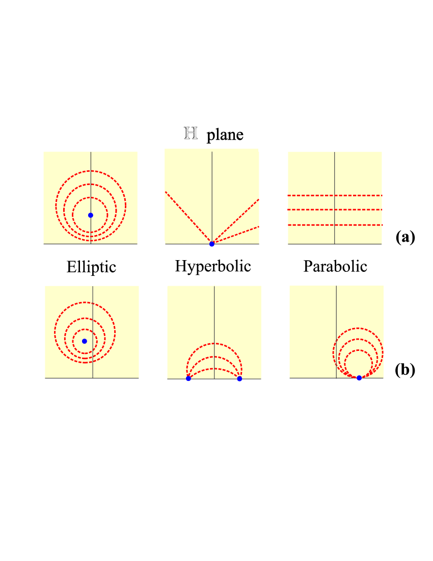
Figure 1: Plot of typical orbits in the hyperbolic plane $\mathbb{H}$: (a) canonical transfer matrices as given in equation (2.13) and (b) arbitrary transfer matrices obtained by matrix conjugation as in equation (2.10).

When one of the parameters $\theta$, $\xi$, or $\nu$ in (2) varies, the transformed points $Q^{\prime}$ describe a curve called the orbit of $Q$ under the action of the corresponding one-parameter subgroup. In figure 1.a we have plotted typical orbits for the canonical forms (2.13). For matrices $\mathbf{K}_{\mathrm{C}}(\vartheta)$ the orbits are circumferences centered at the invariant point $+i$ and passing through $Q$ and $-1/Q$. For $\mathbf{A}_{\mathrm{C}}(\xi)$, they are lines going from 0 to the $\infty$ through $Q$ and they are known as hypercicles. Finally, for matrices $\mathbf{N}_{\mathrm{C}}(\nu)$ the orbits are lines parallel to the real axis passing through $Q$ and they are known as horocycles [42].

For a general matrix $\mathbf{M}$ the corresponding orbits can be obtained by transforming with the appropriate matrix $\mathbf{C}$ the orbits described before. The explicit construction of the family of matrices $\mathbf{C}$ is not difficult: it suffices to impose that $\mathbf{C}$ transforms the fixed points of $\mathbf{M}$ into the ones of $\mathbf{K}_{\mathrm{C}}(\vartheta)$, $\mathbf{A}_{\mathrm{C}}(\xi)$, or $\mathbf{N}_{\mathrm{C}}(\nu)$, respectively. Just to work out an example that will play a relevant role in the forthcoming, we consider a matrix $\mathbf{M}$ representing an elliptic action with one fixed point denoted by $Q_{f}$. Since the fixed point for the corresponding canonical matrix $\mathbf{K}_{\mathrm{C}}(\vartheta)$ is $+i$, the matrix $\mathbf{C}$ we are looking for is determined by

$$\Psi[\mathbf{C},Q_{f}]=i.$$ (2.21)

If the matrix $\mathbf{C}$ is written as

$$\mathbf{C}=\left(\begin{array}[]{cc}C_{1}&C_{2}\\ C_{3}&C_{4}\end{array}\right),$$ (2.22)

the solution of (2.21) is

$$C_{2} = -\frac{C_{1}\mathop{\mathrm{Re}}\nolimits Q_{f}+C_{3}\mathop{\mathrm{Im}}\nolimits Q_{f}}{|Q_{f}|^{2}},$$

$$C_{4} = \frac{C_{1}\mathop{\mathrm{Im}}\nolimits Q_{f}-C_{3}\mathop{\mathrm{Re}}\nolimits Q_{f}}{|Q_{f}|^{2}}.$$

In addition, the condition $\det\mathbf{C}=+1$ imposes

$$C_{3}=\sqrt{\frac{|Q_{f}|^{2}}{\mathop{\mathrm{Im}}\nolimits Q_{f}}-C_{1}^{2}},$$ (2.24)

that, together (2) determines the matrix $\mathbf{C}$ in terms of the free parameter $C_{1}$.

In figure 1.b we have plotted typical examples of such orbits for elliptic, hyperbolic, and parabolic actions. We stress that once the fixed points of the ray-transfer matrix are known, one can ensure that $Q^{\prime}$ will lie in the orbit associated to $Q$.

3 First-order systems as transformations in the Poincaré unit disc $\mathbb{D}$

To complete the geometrical setting introduced in the previous Section, we explore now a remarkable transformation (introduced by Cayley) that maps bijectively the hyperbolic plane $\mathbb{H}$ onto the unit disc, denoted by $\mathbb{D}$. This can be done via the unitary matrix

$$\bm{\mathcal{U}}=\frac{1}{\sqrt{2}}\left(\begin{array}[]{cc}1&i\\ i&1\end{array}\right),$$ (3.1)

in such a way that

$$\bm{\mathcal{M}}=\bm{\mathcal{U}}\ \mathbf{M}\ \bm{\mathcal{U}}^{-1}=\left(\begin{array}[]{cc}\alpha&\beta\\ \beta^{\ast}&\alpha^{\ast}\end{array}\right),$$ (3.2)

where $\bm{\mathcal{M}}$ is a matrix with $\det\bm{\mathcal{M}}=+1$ and whose elements are given in terms of those of $\mathbf{M}$ by

$$\alpha = \frac{1}{2}[(A+D)+i(C-B)]\,,$$

$$\beta = \frac{1}{2}[(B+C)+i(D-A)].$$

In other words, the matrices $\bm{\mathcal{M}}$ belong to the group SU(1, 1), which plays an essential role in a variety of branches in physics. Obviously, the bilinear action induced by these matrices is

$$\mathcal{Q}^{\prime}=\Phi[\bm{\mathcal{M}},\mathcal{Q}]=\frac{\beta^{\ast}+\alpha^{\ast}\mathcal{Q}}{\alpha+\beta\mathcal{Q}},$$ (3.4)

where $\mathcal{Q}$ is the point transformed by (3.1) of the original $Q$:

$$\mathcal{Q}=\frac{Q-i}{1-iQ}.$$ (3.5)

The transformation by $\bm{\mathcal{U}}$ establishes then a one-to-one map between the group SL(2, $\mathbb{R}$) of matrices $\mathbf{M}$ and the group SU(1, 1) of complex matrices $\bm{\mathcal{M}}$, which allows for a direct translation of the properties from one to the other.

It is easy to see that $\mathbb{H}$ maps onto $\mathbb{D}$, as desired. The imaginary axis in $\mathbb{H}$ goes to the $Y$ axis of the disc $\mathbb{D}$ (in both cases, $R=\infty$ and define beam waists). In particular, $Q=+i$ is mapped onto $\mathcal{Q}=0$. The boundary of $\mathbb{H}$ (the real axis) goes to the boundary of $\mathbb{D}$ (the unit circle), and both boundaries represent fully unlimited irradiance distributions (i.e., non-beam solutions).

Since the matrix conjugation (3.2) does not change the trace, the same geometrical classification in three basic actions still holds. In fact, by conjugating with $\bm{\mathcal{U}}$ the canonical forms (2.13), we get the corresponding ones for SU(1, 1):

$$\bm{\mathcal{K}}_{\mathcal{C}}(\vartheta) = \left(\begin{array}[]{cc}\exp(i\vartheta/2)&0\\ 0&\exp(-i\vartheta/2)\end{array}\right)\ ,$$ (3.8)

$$\bm{\mathcal{A}}_{\mathcal{C}}(\xi) = \left(\begin{array}[]{cc}\cosh(\xi/2)&i\,\sinh(\xi/2)\\ -i\,\sinh(\xi/2)&\cosh(\xi/2)\end{array}\right)\ ,$$ (3.11)

$$\bm{\mathcal{N}}_{\mathcal{C}}(\nu) = \left(\begin{array}[]{cc}1-i\,\nu/2&\nu/2\\ \nu/2&1+i\,\nu/2\end{array}\right)\ ,$$ (3.14)

that have as fixed points 0 (elliptic), $+i$ and $-i$ (hyperbolic) and $+i$ (parabolic), respectively. The first matrix represent a rotation in phase space, also called a fractional Fourier transformation, while the second one is sometimes called a hyperbolic expander [32].

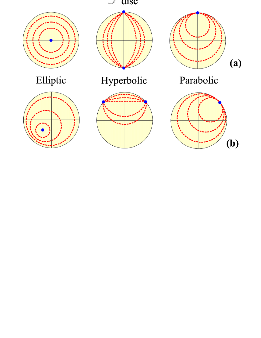
Figure 2: Plot of typical orbits in the Poincaré unit disc $\mathbb{D}$: (a) canonical transfer matrices as given in equation (3.8) and (b) arbitrary transfer matrices.

The corresponding orbits for these matrices are defined by

$$\mathcal{Q}^{\prime} = \Phi[\bm{\mathcal{K}}_{\mathcal{C}},\mathcal{Q}]=\mathcal{Q}\exp(-i\vartheta)\ ,$$

$$\mathcal{Q}^{\prime} = \Phi[\bm{\mathcal{A}}_{\mathcal{C}},\mathcal{Q}]=\frac{\mathcal{Q}-i\tanh(\xi/2)}{1+i\,\mathcal{Q}\tanh(\xi/2)}\ ,$$ (3.15)

$$\mathcal{Q}^{\prime} = \Phi[\bm{\mathcal{N}}_{\mathcal{C}},\mathcal{Q}]=\frac{\mathcal{Q}+(1+i\mathcal{Q})\nu/2}{1+(\mathcal{Q}-i)\nu/2}.$$

As plotted in figure 2.a, for matrices $\bm{\mathcal{K}}_{\mathcal{C}}(\vartheta)$ the orbits are circumferences centered at the origin. For $\bm{\mathcal{A}}_{\mathcal{C}}(\xi),$ they are arcs of circumference going from the point $+i$ to the point $-i$ through $\mathcal{Q}$. Finally, for the matrices $\bm{\mathcal{N}}_{\mathcal{C}}(\nu)$ the orbits are circumferences passing through the points $i$, $\mathcal{Q}$, and $-\mathcal{Q}^{\ast}$. In figure 2.b we have plotted the corresponding orbits for arbitrary fixed points.

4 Application to optical resonators

The geometrical ideas presented before allows one to describe the evolution of a GSM beam by means of the associated orbits. As an application of the formalism, we consider the illustrative example of an optical cavity consisting of two spherical mirrors of radii $R_{1}$ and $R_{2}$, separated a distance $d$. The ray-transfer matrix corresponding to a round trip can be routinely computed [4]

$$\mathbf{M}=\left(\begin{array}[]{cc}2g_{1}g_{2}-g_{1}+g_{2}-1&\displaystyle\frac{d}{2}(2g_{1}g_{2}+g_{1}+g_{2})\\ \displaystyle\frac{2}{d}(2g_{1}g_{2}-g_{1}-g_{2})&2g_{1}g_{2}+g_{1}-g_{2}-1\end{array}\right),$$ (4.1)

where we have used the parameters ($i=1,2$)

$$g_{i}=1-\frac{d}{R_{i}}.$$ (4.2)

Note that

$$\Tr(\mathbf{M})=2(2g_{1}g_{2}-1).$$ (4.3)

Since the trace determines the fixed point and the orbits of the system, the $g$ parameters establish uniquely the geometrical action of the resonator. To clarify further this point, in figure 3 we have plotted the value of $|\Tr(\mathbf{M})|$ in terms of $g_{1}$ and $g_{2}$. The plane $|\Tr(\mathbf{M})|=2$, which determines the boundary between elliptic and hyperbolic action, is also shown. At the top of the figure, a density plot is presented, with the characteristic hyperbolic contours.

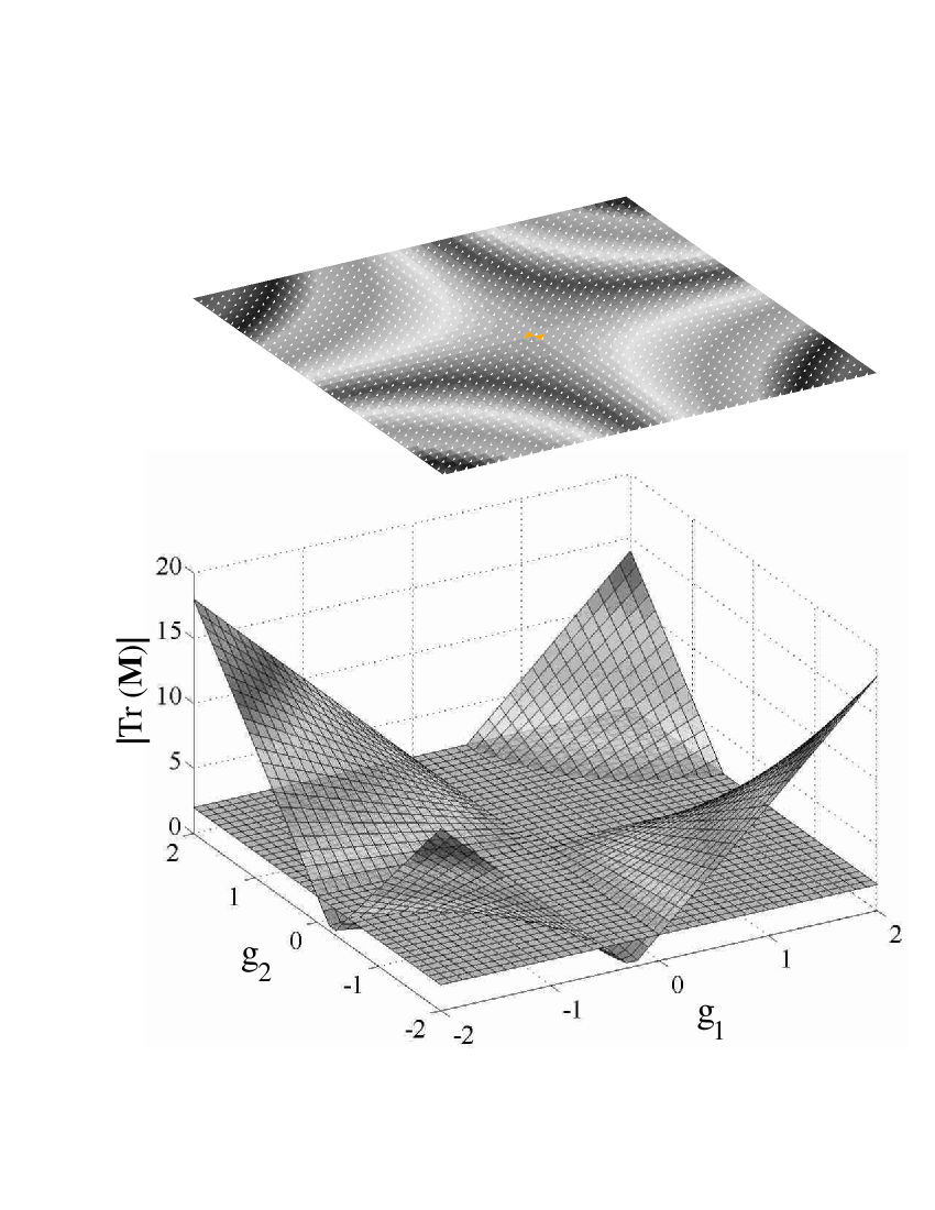
Figure 3: Plot of $|\Tr(\mathbf{M})|$ in terms of the parameters $g_{1}$ and $g_{2}$ of the optical resonator. The plane $|\Tr(\mathbf{M})|=2$ is also shown. The density plot of the three-dimensional figure appears at the bottom.

Assume now that the light bounces $N$ times through this system. The overall transfer matrix is then $\mathbf{M}^{N}$, so all the algebraic task reduces to finding a closed expression for the $N$th power of the matrix $\mathbf{M}$. Although there are several elegant ways of computing this power [21], we shall instead apply our geometrical picture: the transformed beam is represented by the point

$$Q_{N}=\Psi[\mathbf{M},Q_{N-1}]=\Psi[\mathbf{M}^{N},Q_{0}],$$ (4.4)

where $Q_{0}$ denotes the initial point.

Note that all the points $Q_{N}$ lie in the orbit associated to the initial point $Q_{0}$ by the single round trip, which is determined by its fixed points: the character of these fixed points determine thus the behaviour of this periodic system. By varying the parameters $g$ of the resonator we can choose to work in the elliptic, the hyperbolic, or the parabolic case [43].

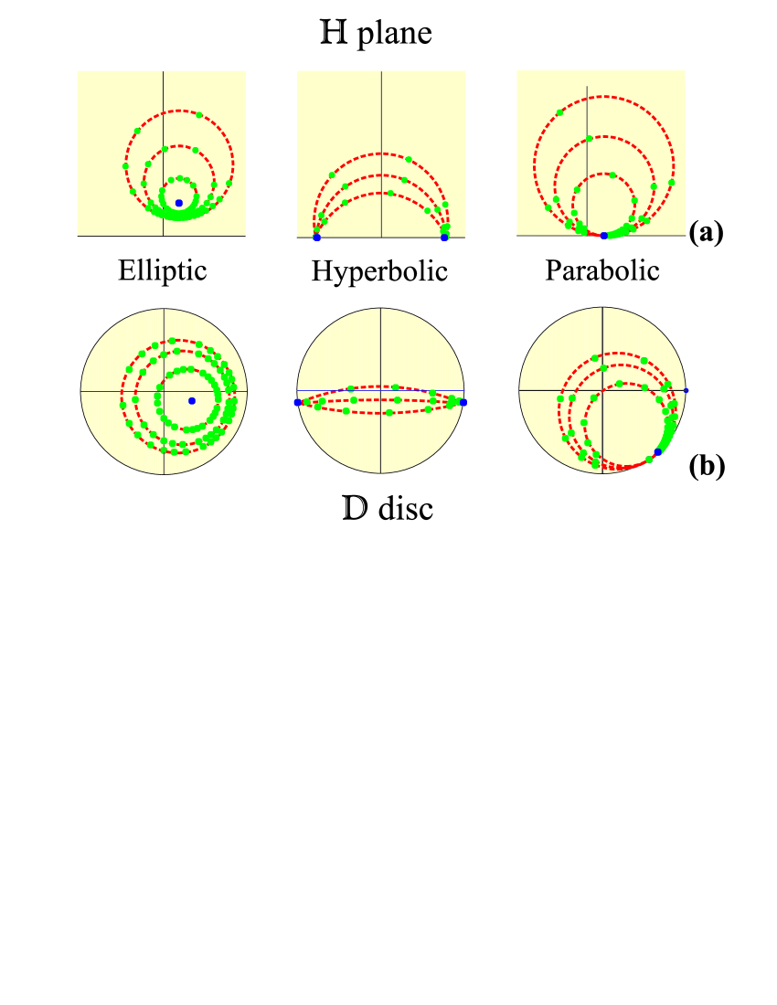
Figure 4: Plot of the successive iterates for typical elliptic, hyperbolic, and parabolic actions. In (a) the points are plotted in the hyperbolic plane $\mathbb{H}$, while in (b) they are represented in the unit disc $\mathbb{D}$. For hyperbolic and parabolic actions, the iterates tend to the real axis and the unit circle, respectively.

To illustrate how this geometrical approach works in practice, in figure 4.a we have plotted the sequence of successive iterates obtained for different kind of ray-transfer matrices, according to our previous classification. In figure 4.b we have plotted the same sequence but in the unit disc, obtained via the unitary matrix $\bm{\mathcal{U}}$.

In the elliptic case, it is clear that the points $Q_{N}$ revolve in the orbit centered at the fixed point and the system never reaches the real axis. Equivalently, the points $\mathcal{Q}_{N}$ never reach the unit circle.

On the contrary, for the hyperbolic and parabolic cases the iterates converge to one of the fixed points on the real axis, although with different laws [44]. In the general context of scattering by periodic systems this corresponds to the band stop and band edges, respectively [45, 46, 47, 48, 49].

What we conclude from this analysis is that the iterates of hyperbolic and parabolic actions produce solutions fully unlimited, which are incompatible with our ideas of a beam. The only beam solutions are thus generated by elliptic actions and, according with equation (4.3), the stability criterion is

$$0\leq|2g_{1}g_{2}-1|=|\cos(\vartheta/2)|\leq 1,$$ (4.5)

where $\vartheta$ is the parameter in the canonical form $\mathbf{K}_{\mathrm{C}}$ in equation (2.13). Such a condition is usually worked out in terms of algebraic arguments using ray-transfer matrices, although the final results apply exclusively to scalar wave fields.

Finally, we stress that real cavities resonate with vector fields. The situation then is far more involved because the vector diffraction for (polarized) electric fields is more difficult to handle, even for systems with small Fresnel numbers and the $ABCD$ law does not apply to the corresponding kernel [50]. Exact solutions for these vector beams have recently appeared [51]. In any case, there is abundant evidence that the stability condition (4.5) works well. This could be expected, since the transition to scalar theories captures all the essential physics embodied in the more elaborated vector analogues [52].

5 Concluding remarks

In this paper, we have provided a geometrical scenario to deal with first-order optical systems. More specifically, we have reduced the action of any system to a rotation, a translation or a parallel displacement, according to the magnitude of the trace of its ray-transfer matrix. These are the basic isometries of the hyperbolic plane $\mathbb{H}$ and also of the Poincaré unit disc $\mathbb{D}$. We have also provided an approach for a qualitative examination of the stability condition of an optical resonator.

We hope that this approach will complement the more standard algebraic techniques and together they will help to obtain a better physical and geometrical feeling for the properties of first-order optical systems.

References

- [1] Hoffman K and Kunze R 1971 Linear Algebra 2nd edition (New York: Prentice Hall)
- [2] Barnett S 1990 Matrices: Methods and Applications (Oxford: Clarendon)
- [3] Kauderer M 1994 Symplectic Matrices: First Order Systems and Special Relativity (Singapore: World Scientific)
- [4] Gerrard A and Burch J M 1975 Introduction to Matrix Methods in Optics (New York: Wiley)
- [5] Wolf E and Collett E 1978 “Partially coherent sources which produce the same far-field intensity distribution as a laser” Opt. Commun. 25 293-6
- [6] Foley J T and Zubairy M S 1978 “The directionality of Gaussian Schell-model beams” Opt. Commun. 26 297-300
- [7] Saleh B E A 1979 “Intensity distribution due to a partially coherent field and the Collett-Wolf equivalence theorem in the Fresnel zone” Opt. Commun. 30 135-8
- [8] Gori F 1980 “Collett-Wolf sources and multimode lasers” Opt. Commun. 34 301-5
- [9] Starikov A and Wolf E 1982 “Coherent-mode representation of Gaussian Schell-model sources and of their radiation fields” J. Opt. Soc. Am. 72 923-8
- [10] Friberg A T and Sudol R J 1982 “Propagation parameters of Gaussian Schell-model beams” Opt. Commun. 41 383-7
- [11] Gori F 1983 “Mode propagation of the field generated by Collett-Wolf Schell-model sources” Opt. Commun. 46 149-54
- [12] Gori F and Grella R 1984 “Shape invariant propagation of polychromatic fields” Opt. Commun. 49 173-7
- [13] Friberg A T and Turunen J 1988 “Imaging of Gaussian Schell-model sources” J. Opt. Soc. Am. A 5 713-20
- [14] Friberg A T, Tervonen E and Turunen J 1994 “Interpretation and experimental demonstration of twisted Gaussian Schell-model beams” J. Opt. Soc. Am. A 11 1818-26
- [15] Ambrosini D, Bagini V, Gori F and Santarsiero M 1994 “Twisted Gaussian Schell-model beams: A superposition model” J. Mod. Opt. 41 1391-99
- [16] Collins S A 1963 “Analysis of optical resonators involving focusing elements” Appl. Opt. 3 1263-75
- [17] Li T 1964 “Dual forms of the gaussian beam chart” Appl. Opt. 3 1315-7
- [18] Kogelnik H 1965 “Imaging of optical modes –resonators with internal lenses” Bell Syst. Tech. J. 44 455-94
- [19] Kogelnik H 1965 “On the propagation of Gaussian beams of light through lenslike media including those with a loss or gain variation” Appl. Opt. 4 1562-9
- [20] Kogelnik H and Li T 1966 “Laser beams and resonators” Appl. Opt. 5 1550-67 and references therein
- [21] Siegman A E 1986 Lasers (Oxford: Oxford University Press)
- [22] Saleh B E A and Teich M C 1991 Fundamentals of Photonics (New York: Wiley)
- [23] Gilmore R 1974 Lie groups, Lie algebras, and some of their Applications (New York: Wiley)
- [24] Krantz S G 1990 Complex Analysis: The Geometric Viewpoint (Providence: American Mathematical Society)
- [25] Simon R, Sudarshan E C G and Mukunda N 1984 “Generalized rays in first-order optics: Transformation properties of Gaussian Schell-model fields” Phys. Rev. A 29 3273-9
- [26] Simon R, Sudarshan E C G and Mukunda N 1985 “Anisotropic Gaussian Schell-model beams: Passage through optical systems and associated invariants” Phys. Rev. A 31, 2419-34
- [27] Simon R, Mukunda N and Sudarshan E C G 1988 “Partially coherent beams and a generalized ABCD-law” Opt. Commun. 65 322-8
- [28] Simon R and Mukunda N 1993 “Twisted Gaussian Schell-model beams” J. Opt. Soc. Am. A 10 95-109
- [29] Simon R and Mukunda N 1998 “Iwasawa decomposition in first-order optics: universal treatment of shape-invariant propagation for coherent and partially coherent beams” J. Opt. Soc. Am. A 15 2146-55
- [30] Wolf K B 2004 Geometric Optics on Phase Space (Berlin: Springer)
- [31] Başkal S, Georgieva E, Kim Y S and Noz M E 2004 “Lorentz group in classical ray optics” J. Opt. B: Quantum Semiclass. Opt.6 S455-72
- [32] Simon R and Wolf K B 2000 “Structure of the set of paraxial optical systems” J. Opt. Soc. Am. A 17, 342-55
- [33] Gloge D and Marcuse D 1969 “Formal quantum theory of light rays” J. Opt. Soc. Am. 59 1629-31
- [34] Dragoman D 1995 “Wigner distribution function for Gaussian Schell beams in complex matrix optical systems” Appl. Opt. 34 3352-7
- [35] Stahl S 1993 The Poincaré half-plane (Boston: Jones and Bartlett)
- [36] Azzam R M A and Bashara N M 1987 Ellipsometry and Polarized Light (Amsterdam: North-Holland) section 4.6
- [37] Han D, Kim Y S and Noz M E 1996 “Polarization optics and bilinear representation of the Lorentz group” Phys. Lett. A 219 26-32
- [38] Sánchez-Soto L L, Monzón J J, Yonte T and Cariñena J F 2001 “Simple trace criterion for classification of multilayers” Opt. Lett. 26 1400-2
- [39] Lekner J 1994 “Light in periodically stratified media” J. Opt. Soc. Am. A 11 2892-9
- [40] Yonte T, Monzón J J, Sánchez-Soto L L, Cariñena J F and López-Lacasta C 2002 “Understanding multilayers from a geometrical viewpoint” J. Opt. Soc. Am. A 19 603-9
- [41] Monzón J J, Yonte T, Sánchez-Soto L L and Cariñena J F 2002 “Geometrical setting for the classification of multilayers” J. Opt. Soc. Am. A 19 985-91
- [42] Coxeter H S M 1969 Introduction to Geometry (New York: Wiley)
- [43] Başkal S and Kim Y S 2002 “Wigner rotations in laser cavities” Phys. Rev. E 026604
- [44] Barriuso A G, Monzón J J and Sánchez-Soto L L 2003 “General unit-disk representation for periodic multilayers” Opt. Lett. 28, 1501-3
- [45] Lekner J 1987 Theory of Reflection (Amsterdam: Dordrecht)
- [46] Yeh P 1988 Optical Waves in Layered Media (New York: Wiley)
- [47] Griffiths D J and Steinke C A 2001 “Waves in locally periodic media” Am. J. Phys. 69 137-154
- [48] Sprung D W L, Morozov G V and Martorell J 2004 “Geometrical approach to scattering in one dimension” J. Phys. A: Math. Gen.37 1861-80
- [49] Sánchez-Soto L L, Cariñena J F, Barriuso A G and Monzón J J 2005 “Vector-like representation of one-dimensional scattering” Eur. J. Phys. 26 469-80
- [50] Hsu H Z and Barakat R 1994 “Stratton-Chu vectorial diffraction of electromagnetic fields by apertures with application to small-Fresnel-number systems” J. Opt. Soc. Am. A 11 623-9
- [51] Lekner J 2001 “TM, TE, and ‘TEM’ beam modes: exact solutions and their problems” J. Opt. A: Pure Appl. Opt.3 407-12
- [52] Mandel L and Wolf E 1995 Optical Coherence and Quantum Optics (Cambridge: Cambridge U. Press)