Coupled-mode theory for periodic side-coupled microcavity and photonic crystal structures

Abstract

We use a phenomenological Hamiltonian approach to derive a set of coupled mode equations that describe light propagation in waveguides that are periodically side-coupled to microcavities. The structure exhibits both Bragg gap and (polariton like) resonator gap in the dispersion relation. The origin and physical significance of the two types of gaps are discussed. The coupled-mode equations derived from the effective field formalism are valid deep within the Bragg gaps and resonator gaps.

I Introduction

In the past several years the linear and nonlinear properties of side-coupled waveguiding structures have attracted the attention of many researchers LittlePaper ^-WaksPaper . These structures consist of one or more waveguiding elements in which forward and backward propagating waves are indirectly coupled to each other via one or more mediating resonant cavities. Perhaps the most common proposals for realizing these structures involve photonic crystal (PC) waveguides with defect modes slightly displaced from the waveguiding region (Fig. 1a, left) HausPaper1 ^,YarivPaper1 , or micro-ring resonator structures in which two channel waveguides are side-coupled to micro-ring resonators (Fig. 1a, right) InvitedPaper . In the PC structure the forward and backward propagating modes within the waveguide are coupled via the defect; for the micro-ring structure, the forward going mode in the lower (upper) channel waveguide is coupled, via the micro-ring, to the backward going mode in the upper (lower) channel. The linear and nonlinear properties of both types of structures have been studied HausPaper1 ^,YarivPaper1 ^-SoljacicPaper .

The electromagnetic properties of these structures can be accurately determined in great detail using numerically intensive methods such as finite-difference time-domain (FDTD) simulations FDTDbook . An analysis in terms of Wannier functions can substantially reduce computation time for the PC structure KurtPaper1 , but the numerical problem remains daunting. In particular, full FDTD calculations of the micro-ring structures have to date been confined to two-dimensional analogs of the actual structures of interest FDTDbook . Furthermore, direct numerical simulation, while valuable for design purposes, offers little insight into the physics of the structures. Consequently, semi-analytical techniques, such as the scattering-matrix approach of S. Fan et al.HausPaper1 and Yong Xu et al.YarivPaper1 , have been proposed. Using these techniques the optical properties of side-coupled structures can be understood in terms of the interactions between a small number of modes.

In this paper we concentrate our attention on periodic, side coupled structures (Fig. 1b). Our primary objective is to derive coupled mode equations (CME) that describe pulse propagation in such structures. Coupled mode theory has long been used as an effective design tool for grating structures where forward and backward propagating waves are directly coupled via an index grating YarivQEBook . In directly coupled structures, it is well known that a Bragg gap opens in the dispersion relation of the structure when the phase accumulated in one round trip through a period of the grating is an integer multiple of $2\pi$, so that the slight reflections that are incurred due to the grating are coherently enhanced. Structures possessing a Bragg gap have found a variety of uses, such as dispersion compensation EggletonPaper and wavelength division multiplexing GilesPaper . In the side-coupled structure the Bragg feedback mechanism, and hence the Bragg gap, does exist, although it is now mediated by the coupling cavity. However, there is also a second type of gap: a resonator gap, which is associated with the resonance frequencies - and therefore the geometry - of the mediating cavity. For the micro-ring resonator structure the interpretation of this gap is straightforward: when the phase accumulated in a round-trip through the micro-ring resonator is an integer multiple of $2\pi$, then the coupling between the forward and backward going waves is resonantly enhanced. Of these two gaps, the resonator gap is perhaps the more important, because it exhibits a deep transmission dip seen even in a structure with only one unit cell.

Because side-coupled structures exhibit both Bragg and resonator gaps, it is to be expected that a CME description of optical pulse propagation will be more complicated than in Bragg gratings. The CME for Bragg gratings involve two fields (forward and backward going) interacting via a coupling coefficient. For side-coupled structures, the most interesting situation is when a resonator gap lies near one of the Bragg gaps, and we show in this paper that the relevant CME then involves three fields: a cavity field and forward and backward going fields.

We derive our CME using a phenomenological Hamiltonian approach, which distills the essential physical interactions of the structure, and hence provides a simple physical picture of optical interactions. We build the fields in our CME as Fourier superpositions of the modes in the Hamiltonian. Hence, our CME are derived for infinite, periodic structures in which the coupling to each cavity is the same. Nevertheless, we show that our CME can be generalized to describe finite, apodized structures, in which the coupling (but not the period) varies from cavity to cavity. Therefore, the CME can be used to describe finite structures with only a small number of cavities. Indeed, the general Hamiltonian approach we advocate can be applied even to structures with only one or two cavities, if the formalism we introduce in Sec. II is extended to a discrete number of (not necessarily identical) cavities. In both discrete and periodic scenarios, the Hamiltonian approach exhibits the similarities of the optical dynamics of these artificially structured materials to more traditional problems in solid state physics. As well, it allows for an easy quantization of the description to address the quantum optics of these structures. We plan to turn to this, as well as the direct derivation of our phenomenological Hamiltonian from the underlying electrodynamics, in future publications.

The present paper is organized as follows. In Sec. II we describe the Hamiltonian model for a system with a single microresonator, investigate the transmission/reflection spectrum of the structure, and indicate how the parameters in our phenomenological Hamiltonian can be set from more common models of cavity resonators. In Sec. III we discuss how the Hamiltonian can be used to model a periodic waveguide-resonator structure. We then discuss methods of reducing the number of fields and interactions in our Hamiltonian while retaining the basic physics. In Sec. IV we derive the coupled mode equations in terms of effective fields built as Fourier superpositions of the modes in the Hamiltonian of Sec. III, and we show how to modify these CME to describe finite, apodized structures. In Sec. V we conclude.

II Hamiltonian model and transmission for a single cavity structure

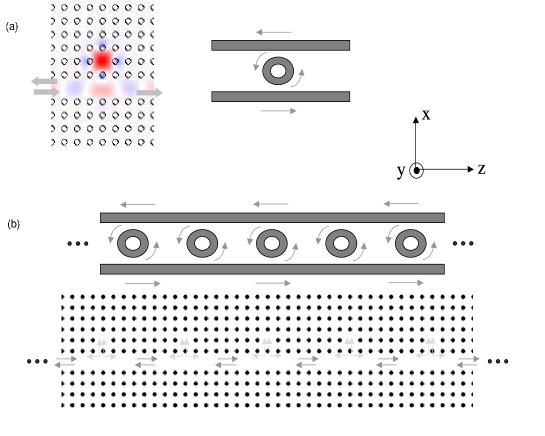
Figure 1: (1a) Waveguide-resonator structure containing (left) photonic crystal microcavity and (right) micro-ring resonator. On the right the micro-ring resonator is coupled to two waveguides, with the forward (backward) propagating light in the lower (upper) waveguide; On the left the structure contains dielectric rods is embedded in air, the singly degenerate microcavity is coupled to the photonic crystal waveguide, formed by removing a row of rods in the photonic crystal. (1b) Periodic waveguide resonator structure containing (top) microring resonator and (bottom) photonic crystal microcavity.

In this section we construct a Hamiltonian model for a structure in which forward and backward propagating waves are indirectly coupled to each other via a cavity centred at $z=z_{0}$. We will focus on classical optics here, but because its easy generalization to quantum optics is one of the strengths of this approach, we adopt a quantum notation and, for the classical Poisson bracket $\left\{..,..\right\}$, we write $(i\hbar)^{-1}\left[..,..\right]$; we also use ^† to indicate complex conjugation. We will also often speak of operators rather than variables, especially when it makes the physics more clear. For example, we introduce $a_{k}^{\dagger}$ and $c_{k}^{\dagger}$ as creation operators for photons propagating with wavenumber $k$ in the forward and backward direction respectively. Because $k>0$ ($k<0$) indicates that the photons are propagating in the forward (backward) direction, $a_{k}^{\dagger}$ exists for $k>0$ and $c_{k}^{\dagger}$ for $k<0$. For a given $k$, the energy in these fields is $\hbar\omega_{k}a_{k}^{\dagger}a_{k}$ and $\hbar\omega_{k}c_{k}^{\dagger}c_{k}$, with $\omega_{k}=c\left|k\right|/n$, where $c$ is the speed of light in a vacuum, and $n$ is a constant effective index, equal for the forward and backward propagating waves. By ignoring the frequency dependence of $n$ we are neglecting the underlying material dispersion within the waveguides; we discuss the validity of this approximation after equation (5) below. To describe light in the cavity, we define a creation operator $b^{\dagger}$, and identify the energy in the field as $\hbar\omega_{0}b^{\dagger}b$, where $\omega_{0}$ is the resonant frequency of the cavity. For the micro-ring resonator structure of Fig. 1a (right), the $a_{k}^{\dagger}$ and $c_{k}^{\dagger}$ could represent creation operators for light propagating in the forward direction in the lower waveguide and the backward direction in the upper waveguide, while $b^{\dagger}$ could represent the field circulating in the counter-clockwise direction in the micro-ring resonator. Our notation implies that the two waveguides have a common mode index $n$, but this could easily be generalized. For the PC structure of Fig. 1a (left), the $a_{k}^{\dagger}$ and $c_{k}^{\dagger}$ would represent creation operators for light propagating in the forward and backward direction in a waveguide mode of the PC waveguide, and $b^{\dagger}$ would represent the creation operator for the field inside the single mode defect. Regardless of their interpretation, the operators satisfy the commutation relations

$$\left[a_{k},a_{k^{\prime}}^{\dagger}\right] = \delta\left(k-k^{\prime}\right),$$

$$\left[c_{k},c_{k^{\prime}}^{\dagger}\right] = \delta\left(k-k^{\prime}\right),$$

$$\left[b,b^{\dagger}\right] = 1,$$ (1)

with all other commutation relations vanishing. Assuming that no light couples directly between the propagating modes governed by $a_{k}^{\dagger}$ and $c_{k}^{\dagger}$, but that light can couple from these modes to the cavity, we use the following model Hamiltonian for the system HausPaper1 ^,YarivPaper1 :

$$H\mathbf{=}H_{o}+H_{coupling},\\$$ (2)

where

$$H_{o} = \int_{0}^{\infty}dk\hbar\omega_{k}a_{k}^{\dagger}a_{k}+\int_{-\infty}^{0}dk\hbar\omega_{k}c_{k}^{\dagger}c_{k}+\hbar\omega_{o}b^{\dagger}b,$$

$$H_{coupling} = -\hbar\int_{0}^{\infty}\xi_{k}\left[a_{k}^{\dagger}be^{-ikz_{0}}+b^{\dagger}a_{k}e^{ikz_{0}}\right]dk$$

$$-\left(-1\right)^{q}\hbar\int_{-\infty}^{0}\xi_{-k}\left[c_{k}^{\dagger}be^{-ikz_{0}}+b^{\dagger}c_{k}e^{ikz_{0}}\right]dk.$$

The quantities $\xi_{k}$ and $\left(-1\right)^{q}\xi_{-k}$ characterize the strength of the coupling between cavity field and waveguide fields, propagating in the forward and backward direction; $q$ is an integer that depends on the symmetry of the cavity mode YarivPaper1 . Note that except for the factor $(-1)^{q}$ our notation implies that the coupling to forward and backward propagating waveguide modes is identical. In the micro-ring structure, for example, this means that we assume equal coupling to the two waveguides; generalization of this is straightforward, but for simplicity we will not do it here. The time evolution of the operators is given by the Heisenberg equations of motion

$$i\hbar\frac{dO}{dt}=\left[O,H\right],$$ (5)

where $O$ is any operator.

In writing down (2), (II) and (LABEL:2_Ham_eqn3) we have implicitly assumed that the cavity supports only one mode, with resonant frequency $\omega_{0}$, and that the waveguides guide light in only a single spatial mode profile. Strictly speaking, of course, neither of these assumptions is valid. In general, cavities support more than one mode, oscillating at one or more resonance frequencies, and for sufficiently high frequencies a waveguide will support multiple transverse modes. However, we are primarily interested in the physics of these structures for frequencies at or near a specific resonant frequency $\omega_{0}$. We then assume that within this frequency range only one resonance of the cavity exists or, alternatively, that only a single mode of a multi-mode cavity is excited, and that the waveguides of the structure are single mode. Furthermore, we assume that the underlying material or modal dispersion of the structure is negligible within the frequency range of interest. For our purposes, the inclusion of material dispersion would lead to quantitative, but not qualitative changes.

In Appendix $1$ we show that our Hamiltonian formulation leads to a Lorentzian transmission and reflection across the cavity for frequencies in the vicinity of $\omega_{0}$:

$$t\left(\omega\right) \simeq \frac{-i\Delta}{\gamma-i\Delta},$$ (6)

$$r\left(\omega\right) \simeq \left(-1\right)^{q}\left(\frac{\gamma}{\gamma-i\Delta}\right),$$ (7)

where $\gamma=2\pi n\xi_{\tilde{\omega}_{0}}^{2}/c$, and $\xi_{\tilde{\omega}_{o}}$ is the coupling coefficient between the cavity and waveguides evaluated at $k=\tilde{\omega}_{0}\equiv n\omega_{0}/c$, and where $\Delta=\left(\omega-\omega_{0}-\alpha\left(\omega\right)\right)$ characterizes the detuning from the renormalized resonance frequency $\omega_{0}+\alpha\left(\omega\right)$ . An expression for the quantity $\alpha\left(\omega\right)$ is given in Appendix $1$. For our structures of interest $\alpha\left(\omega\right)$ is sufficiently small that $\omega-\omega_{0}-\alpha\left(\omega\right)\simeq\omega-\omega_{0}$ to a good approximation.

The transmission and reflection coefficients in (6),(7) are of precisely the form that follows from simple transfer matrix models of resonant cavities or ring resonators YarivPaper1 ^,InvitedPaper . In the latter structure, for example, the coupling of the cavity to the waveguides is described by self-coupling and cross-coupling coefficients $\sigma$ and $\kappa$ respectively, which in a simple case (where the coupling is assumed to occur at the point of smallest separation) are real and satisfy $\sigma^{2}+\kappa^{2}=1$. Comparing the transmission and reflection coefficients found there with (6),(7), we find that they become equivalent if we put

$$\gamma=\frac{c}{2\pi\bar{n}R}\left(\frac{1-\sigma^{2}}{\sigma^{2}}\right)$$ (8)

where $\bar{n}$ and $R$ are the effective index and radius of the resonator respectively. Thus if a given resonator is parameterized by $\sigma$ and $\kappa$, as well of course by the resonance frequency $\omega_{0}$, then relation (8) allows one to determine the effective coupling coefficient $\xi_{\tilde{\omega_{0}}}$ and thus set what will be, as we will see, the crucial elements in the phenomenological Hamiltonian (2). The appropriate values of $\sigma\,$and $\kappa$ for a single resonator could be determined by experiment, or directly calculated from the underlying channel and resonator geometries, as discussed by Waks and Vuckovic WaksPaper .

A typical spectrum for a single cavity structure is shown in Fig. 2. On resonance, the reflection induced by the cavity reaches 100% (albeit only for a single wavelength), and remains significant as long as the detuning, $\Delta$, is on the order of $\gamma$. The width of the spectrum is dictated by $\gamma$, and the larger the coupling to the cavity, the broader the resonance. In physical terms, this means that as the waveguides are brought closer to the cavity of Fig. $1a$, the resonance width increases.

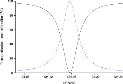
Figure 2: Transmission (solid line) and reflection (dotted line) spectrum for the one cell structure obtained using equations (6) and (7). The structure can demonstrate 100% reflection and 0% transmission when the frequency is matched to the resonance frequency of the microresonator. For comparison with later plots, the frequency is normalized with a distance $\Lambda$, which we use as the distance between resonators when we consider a periodic array.

III Hamiltonian for a periodic structure

We now generalize the single-cavity Hamiltonian to describe a periodic structure, in which the forward and backward propagating modes are coupled to an infinite series of periodically spaced cavities (Fig. 1b). We assume that the resonators are not directly coupled to each other, although of course they do couple indirectly via the waveguides. Generalizing the Hamiltonian (2) to include the periodic sequence of resonators, we write

$$H = \int_{0}^{\infty}dk\hbar\omega_{k}a_{k}^{\dagger}a_{k}+\int_{-\infty}^{0}dk\hbar\omega_{k}c_{k}^{\dagger}c_{k}+\sum_{l}\hbar\omega_{o}b_{l}^{\dagger}b_{l}$$

$$-\hbar\sum_{l}\int_{0}^{\infty}dk\xi_{k}\left[b_{l}^{\dagger}a_{k}e^{ikz_{l}}+a_{k}^{\dagger}b_{l}e^{-ikz_{l}}\right]$$

$$-\left(-1\right)^{q}\hbar\sum_{l}\int_{-\infty}^{0}\xi_{-k}dk\left[b_{l}^{\dagger}c_{k}e^{ikz_{l}}+c_{k}^{\dagger}b_{l}e^{-ikz_{l}}\right],$$

where $a_{k}^{\dagger}$ $\left(c_{k}^{\dagger}\right)$ are again the creation operators for light propagating the forward (backward) direction. The main difference between (III) and (2) is that we have now included a countably infinite number of resonators, each with the same resonance frequency, $\omega_{0}$, and associated with the creation operator $b_{l}^{\dagger}$, where $l$ indexes the resonator. The resonators are evenly spaced at $z_{l}=l\Lambda$, which gives a fundamental reciprocal lattice vector $G_{0}=2\pi/\Lambda$. The Hamiltonian (III) can be re-written as

$$H = \sum_{G}\int_{B.Z.}dk\hbar\omega_{k+G}a_{k+G}^{\dagger}a_{k+G}+\sum_{G}\int_{B.Z.}dk\hbar\omega_{k-G}c_{k-G}^{\dagger}c_{k-G}+\sum_{l}\hbar\omega_{o}b_{l}^{\dagger}b_{l}$$ (10)

$$-\hbar\sum_{l}\sum_{G}\int_{B.Z.}dk\xi_{k+G}\left[b_{l}^{\dagger}a_{k+G}e^{i\left(k+G\right)z_{l}}+a_{k+G}^{\dagger}b_{l}e^{-i\left(k+G\right)z_{l}}\right]$$

$$-\left(-1\right)^{q}\hbar\sum_{l}\sum_{G}\int_{B.Z.}dk\xi_{-k+G}\left[b_{l}^{\dagger}c_{k-G}e^{i\left(k-G\right)z_{l}}+c_{k-G}^{\dagger}b_{l}e^{-i\left(k-G\right)z_{l}}\right],$$

where $\sum_{G}$ represents the summation over an infinite number of positive reciprocal lattice vectors (with $G=0,G_{0},2G_{0},...$), and where in the integrations we restrict the wavenumber $k$ to the first Brillouin zone ($-G_{0}/2<k\leq G_{0}/2$); We sum only over the positive reciprocal lattice vectors so that $a_{k+G}^{\dagger}$ and $c_{k-G}^{\dagger}$ retain their association with forward and backward propagation modes respectively. The operators satisfy commutation relations

$$\left[a_{k+G},a_{k^{\prime}+G^{\prime}}^{\dagger}\right] = \delta\left(k-k^{\prime}\right)\delta_{G,G^{\prime}},$$

$$\left[c_{k-G},c_{k^{\prime}-G^{\prime}}^{\dagger}\right] = \delta\left(k-k^{\prime}\right)\delta_{G,G^{\prime}},$$

$$\left[b_{l},b_{l^{\prime}}^{\dagger}\right] = \delta_{l,l^{\prime}},$$ (11)

with all other commutators vanishing; the first two of these follow immediately from (1). Because the system is periodic, we can identify a countably infinite set of Bragg frequencies in (10). These are the frequencies $\omega_{k\pm G}$ evaluated at $k=0$ or $G_{0}/2$. Hence, since $\omega_{k\pm G}=c\left|k\pm G\right|/n$ for ring resonator structures, the $M^{th}$ Bragg frequency occurs at $\omega_{b}^{(M)}=M\left(cG_{0}/2n\right)$ (with $M\geq 0$ an integer).

To simplify (10), we introduce the collective operator

$$b_{k}=\sqrt{\frac{\Lambda}{2\pi}}\sum_{l}b_{l}e^{-ikz_{l}},$$ (12)

where $k$ is now a continuous variable that ranges over the first Brillouin zone. In Appendix 2 we introduce this operator by first considering only excitations of the resonators periodic over a length $L=N\Lambda$, and then taking $N\rightarrow\infty$. We find in that limit

$$\sum_{l}\hbar\omega_{0}b_{l}^{\dagger}b_{l}\rightarrow\int_{B.Z.}dk\hbar\omega_{o}b_{k}^{\dagger}b_{k},$$

and that

$$\left[b_{k},b_{k^{\prime}}^{\dagger}\right]=\delta\left(k-k^{\prime}\right)$$

for $k$ and $k^{\prime}$ in the first Brillouin zone, with all other commutators vanishing. In terms of this collective operator the Hamiltonian (10) becomes

$$H = \sum_{G}\int_{B.Z.}dk\hbar\omega_{k+G}a_{k+G}^{\dagger}a_{k+G}+\sum_{G}\int_{B.Z.}dk\hbar\omega_{k-G}c_{k-G}^{\dagger}c_{k-G}+\int_{B.Z.}dk\hbar\omega_{o}b_{k}^{\dagger}b_{k}$$ (13)

$$-\hbar\sum_{G}\int_{B.Z.}dk\Xi_{+k+G}\left[b_{k}^{\dagger}a_{k+G}+a_{k+G}^{\dagger}b_{k}\right]-\left(-1\right)^{q}\hbar\sum_{G}\int_{B.Z.}dk\Xi_{-k+G}\left[b_{k}^{\dagger}c_{k-G}+c_{k-G}^{\dagger}b_{k}\right],$$

where $\Xi_{\pm k\pm G}$ $\equiv\sqrt{\frac{2\pi}{\Lambda}}\xi_{\pm k\pm G}$. In Table I we give typical values for parameters characterizing side-coupled structures, and we use them in our sample calculations below. There and for the rest of this paper we assume that the coupling $\Xi_{\pm k\pm G^{\prime}}$ is approximately constant at wavevectors corresponding to frequencies within our region of interest, and take $\Xi_{\pm k\pm G^{\prime}}\approx\Xi$. This approximation is reasonable if the $G$ of interest satisfy $G\ll\Delta k$, where $\Delta k$ is the range over which the $\xi_{k}$ varies significantly. We can expect $\Delta k\approx 2\pi/(1\mu m)$ for the structures of interest (see Appendix 1), and since $G$ is at most a few times $G_{0}=2\pi/\Lambda$ ($=2\pi/(32\mu m)$ from Table I), this inequality is indeed satisfied.

The dispersion relation of the system can be determined by traditional transfer matrix methods, using (6), (7) for the transmission and reflection coefficients of a single resonator. However, to see the connection with the coupled mode equations we will derive, we consider determining the dispersion relation directly from the Hamiltonian (13), by applying the Heisenberg equation of motion to generate equations for the time derivatives of $a_{k+G}$, $c_{k-G}$ and $b_{k}$. Assuming harmonic time dependence $e^{-i\omega t}$ for the operators, we determine an expression for $\omega$ as a complicated function of the countably infinite set of $\omega_{\pm\left|k\right|\pm G}$, and the discrete value $\omega_{0}$. Alternately (and equivalently) we can exhibit the Hamiltonian in a matrix form (13)

$$H=\hbar\int_{BZ}dk\ \mathbf{f}_{k}^{\dagger}\cdot\mathsf{V}_{k}\cdot\mathbf{f}_{k},$$ (14)

where

$$\mathbf{f}_{k}^{\dagger}=\left(a_{k+G_{0}}^{\dagger},a_{k+2G_{0}}^{\dagger},...,c_{k-G_{0}}^{\dagger},c_{k-2G_{0}}^{\dagger},...,b_{k}^{\dagger}\right),$$ (15)

and $\mathsf{V}_{k}$ contains all of the interactions between the $a_{k+G}$, $c_{k-G}$ and $b_{k}$. Then, by diagonalizing the (infinite-dimensional) matrix $\mathsf{V}_{k}$ we can in principle determine the dispersion relation of the structure. In Fig. 3 we consider a typical uncoupled (in the limit where $\Xi=0$) and coupled dispersion relation for the structure. The dotted line shows the uncoupled dispersion relation, and the solid line shows the dispersion relation of the coupled system, as determined by the transfer matrix approach.

Table 1: Parameters used for dispersion relation calculation.

Physical parameters	$\sigma=0.98$	$\Lambda=32.0\mu m$	$n=3.0$	$2\pi R=26.3\mu m$
Numerical parameters	$\frac{\Xi}{c}=0.0023\mu m^{-1}$	$\frac{\omega_{0}n\Lambda}{\pi c}=124.156$	$\frac{\omega_{b}n\Lambda}{\pi c}=124.0$	$\frac{\Xi n\Lambda}{\pi c}=0.07\begin{tabular}[]{lllll}\\ \end{tabular}$

If one of the Bragg frequencies is close to the resonant frequency $\omega_{0}$, then we show below that a truncation of the matrix V_k to three terms is a good approximation. The restricted Hamiltonian that results is

$$H\simeq\hbar\int_{B.Z.}dk\left[\begin{array}[]{lll}a_{k+G^{\prime}}^{\dagger}&c_{k-G^{\prime}}^{\dagger}&b_{k}^{\dagger}\end{array}\right]\left[\begin{array}[]{lll}\omega_{k+G^{\prime}}&0&\Xi\\ 0&\omega_{k-G^{\prime}}&\left(-1\right)^{q}\Xi\\ \Xi&\left(-1\right)^{q}\Xi&\omega_{0}\end{array}\right]\left[\begin{array}[]{l}a_{k+G^{\prime}}\\ c_{k-G^{\prime}}\\ b_{k}\end{array}\right].$$ (16)

where $G^{\prime}$ is the reciprocal lattice vector associated with the forward (backward) band that has $\omega_{k+G^{\prime}}$ $(\omega_{k-G^{\prime}})$ closest to $\omega_{0}$. Here we have assumed that the resonant frequency is very close to a Bragg frequency with its associated gap at the Brillouin zone centre, and so $\omega_{G^{\prime}}=\omega_{-G^{\prime}}\equiv\omega_{b}$, where $\omega_{b}$ is the Bragg frequency closest to the resonance frequency⁸. We refer to eqn. 16 as the “three mode model.” Its validity near a resonance frequency for any particular structure can be formally investigated by including the omitted terms in a multiple scales analysis, or by simply comparing the dispersion relation following from eqn. 16 with a full solution of the dispersion relation using a transfer matrix approach. This is done in Fig. 4, using the parameters in Table I as was done in Fig. 3. In Fig. 4 we also plot the imaginary part of $k$ within the gaps. Note that the exact solution and that from the three mode model are in good agreement for the frequency range shown in Fig. 4. Such agreement fails at other Bragg frequencies that are further from the resonant gap, of course, since the three mode model (eqn. 16) only contains the physics of the Bragg gap closest to $\omega_{0}$. It is to frequencies near $\omega_{0}$ that we henceforth restrict ourselves.

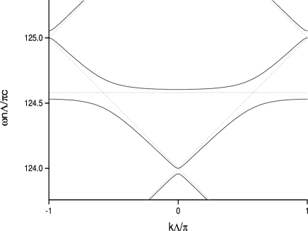
Figure 3: Typical dispersion relation for coupled microresonator system as depicted in Fig. 1 (solid line). For comparison, the dispersion relation of the system in the limit of no coupling (dotted line) is also shown. The resonance frequency of the cavity is given by $\omega_{0}n\Lambda/\pi c=124.58$

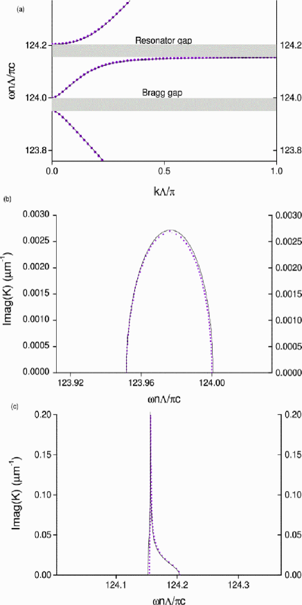
Figure 4: Dispersion relation obtained using the transfer matrix technique (solid line) and the Hamiltonian in (16) (circles). (a) The real part of the dispersion relation. (b) The imaginary part of the wavenumber for frequencies within the Bragg gap (c) The imaginary part of the wavenumber for frequency within the resonator gap.

IV Coupled-mode equations in the three-mode model

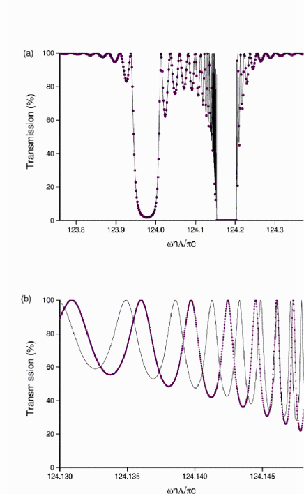
Figure 5: Transmission spectrum for finite structure that contains 30 cavities, using parameters depicted in Table I. (a) Solid line represents the transmission spectrum obtained using coupled mode equations and circles represents the transmission spectrum obtained using transfer matrix. (b) Transmission spectrum in the vicinity of the resonator gap using coupled mode equations (solid line) and transfer matrix (solid line with circles).

In this section we derive a set of coupled-mode equations which describe pulse propagation in the periodic structure, based on the three-mode Hamiltonian (16). We then demonstrate that although these coupled mode equations are derived for an infinite periodic system with equal coupling at each resonator, they can, with only slight modifications, be used to describe finite systems with varying coupling at each resonator. We start by defining effective fields in terms of the amplitudes $a_{k+G^{\prime}}$, $c_{k-G^{\prime}}$ and $b_{k}$:

$$g_{+}\left(z,t\right) = \int_{B.Z.}\frac{dk}{\sqrt{2\pi}}a_{k+G^{\prime}}e^{ikz},$$

$$g_{-}\left(z,t\right) = \int_{B.Z.}\frac{dk}{\sqrt{2\pi}}c_{k-G^{\prime}}e^{ikz},$$

$$b\left(z,t\right) = \int_{B.Z.}\frac{dk}{\sqrt{2\pi}}b_{k}e^{ikz}.$$ (17)

where $G^{\prime}$ indexes the reciprocal lattice vector that is retained within the three mode approximation. These fields can be interpreted as a forward propagating field, a backward propagating field, and the field distribution in the resonators respectively. Using the definitions in (17), the effective fields satisfy the equal time commutation relations,

$$\left[g_{\pm}\left(z,t\right),g_{\pm}^{\dagger}\left(z^{\prime},t\right)\right] = \hat{\delta}\left(z-z^{\prime}\right)$$

$$\left[b\left(z,t\right),b^{\dagger}\left(z^{\prime},t\right)\right] = \hat{\delta}\left(z-z^{\prime}\right),$$ (18)

with all other commutation relations vanishing. The function $\hat{\delta}(z-z^{\prime})$ is an effective delta function such that $\int_{-\infty}^{\infty}f(z)\hat{\delta}(z-z^{\prime})dz=f(z^{\prime})$ when the function $f(z)$ has its wavenumber restricted to the first Brillouin zone of the system. In terms of the effective fields, the Hamiltonian in (16) becomes

$$H = \hbar\omega_{b}\int dzg_{+}g_{+}^{\dagger}+i\frac{\hbar c}{2n}\int dz\left(\frac{\partial g_{+}^{\dagger}}{\partial z}g_{+}-g_{+}^{\dagger}\frac{\partial g_{+}}{\partial z}\right)$$ (19)

$$+ \hbar\omega_{b}\int dzg_{-}g_{-}^{\dagger}-i\frac{\hbar c}{2n}\int dz\left(\frac{\partial g_{-}^{\dagger}}{\partial z}g_{-}-g_{-}^{\dagger}\frac{\partial g_{-}}{\partial z}\right)$$

$$+ \hbar\omega_{0}\int dzbb^{\dagger}-\hbar\Xi\int dz\left(b^{\dagger}g_{+}+c.c.\right)$$

$$- \left(-1\right)^{q}\hbar\Xi\int dz\left(b^{\dagger}g_{-}+c.c.\right)$$

where $\omega_{b}$ denotes the Bragg frequency centered at the Brillouin zone center and closest to $\omega_{0}$ Bragg_definition . Using the Heisenberg equations of motion for the effective fields, we obtain the coupled equations

$$\left(\frac{\partial}{\partial t}+\frac{c}{n}\frac{\partial}{\partial z}\right)g_{+}\left(z,t\right) = -i\omega_{b}g_{+}\left(z,t\right)+i\Xi b\left(z,t\right),$$

$$\left(\frac{\partial}{\partial t}-\frac{c}{n}\frac{\partial}{\partial z}\right)g_{-}\left(z,t\right) = -i\omega_{b}g_{-}\left(z,t\right)+i\left(-1\right)^{q}\Xi b\left(z,t\right),$$

$$\frac{\partial}{\partial t}b\left(z,t\right)=-i\omega_{o}b\left(z,t\right) + i\Xi g_{+}\left(z,t\right)+i\left(-1\right)^{q}\Xi g_{-}\left(z,t\right).$$

One can obtain the dispersion relation directly from (IV) by assuming that each field is a plane wave $e^{ikz-i\omega t}$, with $k$ restricted to the first Brillouin zone. The results are equivalent to those in Fig.4, obtained by diagonalizing (16).

Although the CME (IV) were derived assuming an infinite medium, they can be used to describe a structure where the coupling constant $\Xi$ varies slowly over a distance on the order of the spacing between the resonators. A multiple scale analysis can be used to identify this limit and corrections to it. A more striking inhomogeneous structure is one beginning with a region where there are no resonators, followed by a length $L$ over which resonators are placed with an equal spacing and equal coupling to the channel(s), followed by a region where again there are no resonators. A simple model for such a region would be to use the equations (IV), but replacing $\Xi$ with a position dependent coupling constant $\left[\theta\left(z\right)-\theta\left(z-L\right)\right]\Xi,$ where $\theta$ is the usual step function. It can be easily seen that this model formally violates our assumptions. Consider, for example, fields with a stationary time dependence, so $g_{+}\left(z,t\right)=g_{+}\left(z\right)e^{-i\bar{\omega}t}$, and similarily for all other fields. Then the first equation gives

$$-i\bar{\omega}g_{+}\left(z\right)+\frac{c}{n}\frac{\partial}{\partial z}g_{+}\left(z\right)=-i\omega_{b}g_{+}\left(z\right)+i\left[\theta\left(z\right)-\theta\left(z-L\right)\right]\Xi b\left(z,t\right),$$ (21)

where in fact the factor $\left[\theta\left(z\right)-\theta\left(z-L\right)\right]$ could be omitted, since the third of (IV) together with the position dependent coupling constant guarantees that $b\left(z\right)$ will only be nonzero in the region between $z=0$ and $z=L$. Note however that at $z=0$ and $z=L$ the equation (21) leads to a discontinuous $\partial g_{+}\left(z\right)/\partial z$ if it is assumed that $g_{+}(z)$ is everywhere continuous. This violates, of course, the assumption that fields such as $g_{+}\left(z,t\right)$ are of the form (17).

Despite such a formal violation of our assumptions, this simple model in fact gives a good description of the optical response of a finite structure. To see this, consider first the fields $g_{\pm}(z,t)$ within the structure. It is clear from (IV) that for a supposed frequency $\overline{\omega}$ there are two Bloch wavenumbers, which equivalently follow from (16); they are given by $k\left(\bar{\omega}\right)=\pm\bar{k}$, where

$$\bar{k}=\frac{n}{c}\sqrt{\frac{\left(\Delta_{o}\Delta_{1}-\Xi^{2}\right)^{2}-\Xi^{4}}{\Delta_{0}^{2}}}.$$ (22)

In the equation above $\Delta_{0}=\left(\bar{\omega}-\omega_{0}\right)$ is the detuning from the resonance frequency and $\Delta_{1}=\left(\bar{\omega}-\omega_{b}\right)$ is the detuning from the Bragg frequency that lies closest to $\omega_{0}$. As a result, one can write the forward and backward propagating effective fields, $g_{\pm}\left(z,t\right)$, as

$$g_{\pm}\left(z,t\right) = g_{\pm}\left(z\right)e^{-i\bar{\omega}t}$$

$$g_{\pm}\left(z\right) = g_{\pm}^{\left(1\right)}e^{i\bar{k}z}+g_{\pm}^{\left(2\right)}e^{-i\bar{k}z},$$ (23)

Once $g^{(1)}_{+}$ and $g^{(2)}_{+}$ are set, $g^{(1)}_{-}$ and $g^{(1)}_{-}$ are determined by the dispersion relation, or equivalently (IV). Hence there are only two independent constants. Outside the structure ($\Xi=0$) there are also two independent constants in each of the regions $z<0$ and $z>L$, but the solution of (IV) is simpler. There it takes the form

$$g_{\pm}(z,t) = g_{\pm}(z)e^{-i\bar{\omega}t}$$

$$g_{+}(z) = g_{+}e^{iqz}$$

$$g_{-}(z) = g_{-}e^{-iqz},$$

where $g_{+}$, $g_{-}$ are independent and $q=\bar{\omega}n/c$. For $z<0$ we denote the constants by $g^{<}_{+}$ and $g^{<}_{-}$, and for $z>L$ we denote them by $g^{>}_{+}$ and $g^{>}_{-}$. Now we consider the boundary condition at $z=L$, and note that since no field is incident from $z>L$, we have $g^{>}_{-}=0$; an incident field is specified by $g^{<}_{+}$. Our independent unknowns are then $g^{<}_{-},g^{>}_{+}$, and the constants $g^{(1)}_{+}$ and $g^{(2)}_{+}$ that specify the field in the structure. We solve for these four unknowns by requiring the continuity of $g_{\pm}(z)$ at $z=0$ and $z=L$. The resulting transmittance of the structure can be written as

$$T\left(\omega\right)=\left|\frac{g^{>}_{+}e^{iqL}}{g_{+}^{(1)}+g_{+}^{(2)}}\right|^{2}$$ (24)

with

$$g_{+}^{\left(1\right)} = \frac{e^{-i\bar{k}L}}{2}\left[1+\frac{\Xi^{2}}{\bar{k}\Delta_{o}}\left(\frac{\Delta_{o}\Delta_{1}}{\Xi^{2}}-1\right)\right]g^{>}_{+}e^{iqL},$$

$$g_{+}^{\left(2\right)} = \frac{e^{i\bar{k}L}}{2}\left[1-\frac{\Xi^{2}}{\bar{k}\Delta_{o}}\left(\frac{\Delta_{o}\Delta_{1}}{\Xi^{2}}-1\right)\right]g^{>}_{+}e^{iqL}.$$

In Fig. 5 we compare the transmission spectrum of a two channel micro-ring resonator structure with 30 cavities, calculated both using the transfer matrix technique,⁷ and using the coupled mode equation result eqn. 24. Again we adopt the parameters of Table I. Generally there is good qualitative agreement, with the main features of the spectrum well described by the coupled mode equation result (24), although as noted above it is being applied beyond its strict range of applicability. An extension of this approach leads to the use of the CME (20) to treat a finite structure where the coupling constant $\Xi$ varies from one resonator to the next. To describe this we simply allow $\Xi$ in (20) to adopt a $z$-dependence,

$$\left(\frac{\partial}{\partial t}+\frac{c}{n}\frac{\partial}{\partial z}\right)g_{+}\left(z,t\right) = -i\omega_{b}g_{+}\left(z,t\right)+i\Xi\left(z\right)b\left(z,t\right),$$

$$\left(\frac{\partial}{\partial t}-\frac{c}{n}\frac{\partial}{\partial z}\right)g_{-}\left(z,t\right) = -i\omega_{b}g_{-}\left(z,t\right)+i\left(-1\right)^{q}\Xi\left(z\right)b\left(z,t\right),$$

$$\frac{\partial}{\partial t}b\left(z,t\right)=-i\omega_{0}b\left(z,t\right) + i\Xi\left(z\right)g_{+}\left(z,t\right)+i\left(-1\right)^{q}\Xi\left(z\right)g_{-}\left(z,t\right).$$ (25)

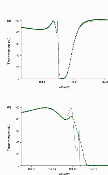
Figure 6: Transmission spectrum for short, finite, apodized structure with 5 unit cells. (a) Solid line represents the transmission spectrum obtained using transfer matrix and squares represent transmission spectrum obtained using coupled mode equations. (b) Transmission spectrum in the vicinity of the resonator gap using transfer matrix (solid line) and coupled mode equations (solid line with squares).

In Fig. 6 we plot the transmission spectrum for a 5 cavity structure apodized such that the cavities (from left to right) are characterized by coupling constants $(\sigma_{1},...\sigma_{5})=(0.993,0.986,0.98,0.986,0.993)$, corresponding to $(\Xi_{1}\Lambda n/\pi c,..\Xi_{5}\Lambda n/\pi c)=(0.0208,0.0287,0.0351,0.0287,0.0208)$. The transfer matrix results is presented, as well as a very simple application of the CME (25) using a piecewise uniform function to represent $\Xi$, where in the $n^{th}$ unit well we set $\Xi=\Xi_{n}$. Again there is good qualitative agreement, although the CME are being applied beyond their strict range of applicability. Besides the difference between the CME and transfer matrix results with respect to the Fabry-Perot type oscillations, as seen in Fig. 5, here the CME solution also consistently overestimates the transmission on the high-frequency side of the stop gap. This can be traced back to the effects on the band curvature induced by the next highest Bragg gap, which are implicitly included in the transfer matrix solution but not in the CME calculation.

Finally, we note that while at least three coupled mode equations are necessary to describe the kind of structures we consider here if we deal with both their space and time dependence, if we instead restrict ourselves to a stationary time dependence, $g_{\pm}\left(z,t\right)=g_{\pm}\left(z\right)e^{-i\bar{\omega}t}$ and $b(z,t)=b(z)e^{-i\bar{\omega}t}$, then in fact we can eliminate the variable $b\left(z,t\right)$ and construct coupled mode equations involving only $g_{+}\left(z,t\right)$ and $g_{-}\left(z,t\right)$. They are

$$\frac{\partial}{\partial z}g_{+}\left(z\right) = i\nu\left(\omega\right)g_{+}\left(z\right)+i\left(-1\right)^{q}\mu\left(\omega\right)g_{-}\left(z\right),$$

$$\frac{\partial}{\partial z}g_{-}\left(z\right) = -i\nu\left(\omega\right)g_{-}\left(z\right)-i\left(-1\right)^{q}\mu\left(\omega\right)g_{+}\left(z\right),$$

where

$$\nu\left(\omega\right) = \frac{n}{c}\left[\frac{\Xi^{2}}{\left(\omega_{0}-\omega\right)}-\left(\omega_{b}-\omega\right)\right],$$

$$\mu\left(\omega\right) = \frac{n}{c}\frac{\Xi^{2}}{\left(\omega_{0}-\omega\right)},$$ (27)

These equations are valid for $\omega\neq\omega_{0}$. It is well-known that a photonic band gap opens in the dispersion relation described by these equations when $\left|\mu\left(\omega\right)\right|\geq\left|\nu\left(\omega\right)\right|$, ProgInOptics and that the width of the gap is larger for larger values of $\left|\mu\left(\omega\right)\right|$. Consequently we see from these equations an analytic confirmation of features that our dispersion relation display. Within our three mode model, one edge of the resonator gap occurs at $\omega\rightarrow\omega_{0}$ (in which case $\nu$ and $\mu$ both diverge equally quickly and are hence equal in the limit as $\omega$ approaches $\omega_{0}$), and one edge of the Bragg gap occurs at $\omega\rightarrow\omega_{b}$, because then the second term in the expression for $\nu\left(\omega\right)$ vanishes, and $\nu\left(\omega_{b}\right)=\mu\left(\omega_{b}\right)$.

V Conclusion

We have presented a phenomenological Hamiltonian description of light propagation in side-coupled resonators. This formulation is appealing in its simplicity, since it captures the basic physics of the structures via a set of readily understandably parameters. The most interesting special case is perhaps where a resonator gap is close to a Bragg gap, and at frequencies close to these gaps a three mode model gives a good description of the dynamics of a periodic structure of resonators. Coupled mode equations based on these captures the dispersion relation even deep within the gaps, and a naive extension of these equations to describe finite structures, although not within the strict range of applicability of the model, gives a good qualitative description.

A hallmark of the kind of approach we have taken here is the connection of theoretically calculated or experimentally observed parameters, such as the coupling coefficient $\sigma$, to the parameters that appear in our phenomenological Hamiltonian. Such a strategy is particularly amenable to the description of quantum and nonlinear optical effects. The Hamiltonian description leads to straightforward quantization, of course, and appropriate nonlinear terms can easily be added to the Hamiltonian. In a previous study by Grimshaw et al.²², it was shown that three nonlinear coupled mode equations support stationary solitary wave solution in the presence of Kerr nonlinearity. Numerical studies have indicated that soliton-like waves exist in resonator structures. In future work we plan to apply the approach we have detailed here to study such field excitations, where a Hamiltonian framework provides the ability to characterize conserved quantities in terms of the symmetries of the nonlinear field theory.

VI Acknowledgments

This project was partly funded by the Natural Science and Engineering Research Council (NSERC) of Canada. Philip Chak acknowledges financial support from Photonic Research Ontario and an Ontario Graduate Scholarship.

VII Appendix 1

In this appendix we use the Hamiltonian (2) to determine the transmission properties of a single-cavity structure. These transmission properties have been intensively studied using various methods such as finite difference, time domain simulationsFDTDbook , and scattering matrix techniquesHausPaper1 YarivPaper1 , and it is well-known that a Lorentzian function gives an excellent approximation to the response of the structure. Here we show that our Hamiltonian also leads to a Lorentzian spectrum. To discuss transmission and reflection, we assume that there is a time-dependent source, $u\left(t\right)$, coupled to the forward propagating modes at $z_{s}<z_{0}$. We therefore modify the Hamiltonian (2) to include a source term:

$$H\mathbf{=}H_{o}+H_{coupling}+H_{source},$$ (28)

with

$$H_{source}=-\hbar\int_{0}^{\infty}\left[a_{k}^{\dagger}u\left(t\right)e^{-ikz_{s}}+a_{k}u^{*}\left(t\right)e^{ikz_{s}}\right]dk,$$ (29)

where $e^{ikz_{s}}$ accounts for the fact that the light is generated at $z=z_{s}$. Using the Hamiltonian (28) and the commutation relations (1) in the Heisenberg equations of motion (5) we find

$$a_{k}(t) = i\xi_{k}\int_{-\infty}^{t}b\left(t^{\prime}\right)e^{-i\omega_{k}\left(t-t^{\prime}\right)}e^{-ikz_{o}}dt^{\prime}$$

$$+ i\int_{-\infty}^{t}u\left(t^{\prime}\right)e^{-i\omega_{k}\left(t-t^{\prime}\right)}e^{-ikz_{s}}dt^{\prime},$$

$$c_{k}(t) = i\left(-1\right)^{q}\xi_{-k}\int_{-\infty}^{t}b\left(t^{\prime}\right)e^{-i\omega_{k}\left(t-t^{\prime}\right)}e^{-ikz_{o}}dt^{\prime},$$

$$\frac{db(t)}{dt} = -i\omega_{o}b(t)+i\int_{0}^{\infty}\xi_{k}a_{k}(t)e^{ikz_{o}}dk$$ (30)

$$+ i\left(-1\right)^{q}\int_{-\infty}^{0}\xi_{-k}c_{k}(t)e^{ikz_{o}}dk.$$

where we have formally integrated the Heisenberg equations for $da_{k}/dt$ and $dc_{k}/dt$, so that both $a_{k}\left(t\right)$ and $c_{k}\left(t\right)$ are expressed entirely in terms of $b\left(t\right)$ and $u\left(t\right)$. Using the expressions for $a_{k}\left(t\right)$ and $c_{k}\left(t\right)$ in the equation for $db/dt$, and expanding $b\left(t\right)$ and $u\left(t\right)$ in terms of Fourier components,

$$b\left(t\right) = \frac{1}{2\pi}\int_{-\infty}^{\infty}b\left(\omega\right)e^{-i\omega t}d\omega,$$

$$u\left(t\right) = \frac{1}{2\pi}\int_{-\infty}^{\infty}u\left(\omega\right)e^{-i\omega t}d\omega,$$ (31)

we obtain

$$b\left(\omega\right)=\left[\frac{-2\pi n\xi_{\widetilde{\omega}}/c}{2\pi n\xi_{\widetilde{\omega}}^{2}/c-i\Delta}\right]u\left(\omega\right)e^{i\widetilde{\omega}\left(z_{o}-z_{s}\right)},$$ (32)

where $\Delta=\left(\omega-\omega_{o}+\alpha\left(\omega\right)\right)$ and $\tilde{\omega}=\omega n/c$, with

$$\alpha\left(\omega\right)=2\int_{0}^{\infty}\wp\left(\frac{{\xi}_{k}^{2}}{\frac{c}{n}k-\omega}\right)dk$$ (33)

describing the small shift in the resonance frequency of the cavity due to the presence of the waveguide. To estimate the effect of $\alpha(\omega)$, we assume $\xi_{k}$ takes a gaussian form in k space with a peak centered at $k=\tilde{\omega_{0}}$. We take the width of the gaussian profile to be about $~{}1\mu m^{-1}$, associated with a typical length over which the coupling between the waveguide and resonator is significant. Using this approximate form for $\xi_{k}$ in the expression for $\alpha(\omega)$ and numerically evaluating the integral, we have verified that $\alpha(\omega)$ is much smaller than the resonance frequency $\omega_{0}$ for structures of interest. Note that in (32) we have switched our notation for wavenumber from $k$ to $\widetilde{\omega}=n\omega/c=\left|k\right|$ to stress that we are now considering the frequency response of the structure. To determine the transmission and reflection spectrum of the structure we define a set of effective fields

$$f_{+}\left(z,t\right) = \frac{1}{\sqrt{2\pi}}\int_{0}^{\infty}dka_{k}\left(t\right)e^{ikz},$$

$$f_{-}\left(z,t\right) = \frac{1}{\sqrt{2\pi}}\int_{-\infty}^{0}dkc_{k}\left(t\right)e^{ikz}.$$ (34)

We then substitute the values (30) for $a_{k}\left(t\right)$ and $c_{k}\left(t\right)$ in the effective fields (34), and use the Fourier transforms (31) of $b\left(t\right)$ and $u\left(t\right)$ to simplify the integrals. We are specifically interested in the following two quantities

$$\lim_{z\rightarrow\infty}f_{+}\left(z,t\right) = \frac{i}{c}\int_{0}^{\infty}\left[\frac{-i\Delta}{2\pi n\xi_{\tilde{\omega}}^{2}/c-i\Delta}\right]u\left(\omega\right)e^{ik\left(z-z_{s}\right)}e^{-i\omega t}d\omega,$$ (35)

$$\lim_{z\rightarrow-\infty}f_{-}\left(z,t\right) = \frac{i}{c}\left(-1\right)^{q}\int_{0}^{\infty}\left[\frac{2\pi n\xi_{\tilde{\omega}}^{2}/c}{2\pi n\xi_{\tilde{\omega}}^{2}/c-i\Delta}\right]u\left(\omega\right)e^{ik\left(z+z_{s}\right)}e^{i2\tilde{\omega}z_{o}}e^{-i\omega t}d\omega.$$

Note that in the absence of coupling we would have

$$\lim_{z\rightarrow\infty}f_{+}\left(z,t\right) = \frac{i}{c}\int_{0}^{\infty}u\left(\omega\right)e^{ik\left(z-z_{s}\right)}e^{-i\omega t}d\omega,$$ (36)

$$\lim_{z\rightarrow-\infty}f_{-}\left(z,t\right) = 0$$

The first (second) of the expressions in (35) is the transmitted (reflected) field built as a superposition of the Fourier components of the source term, $u\left(\omega\right)$. We can therefore define the transmission and reflection coefficients as

$$t\left(\omega\right) = \frac{-i\Delta}{2\pi n\xi_{\tilde{\omega}}^{2}/c-i\Delta},$$

$$r\left(\omega\right) = \left(-1\right)^{q}\frac{2\pi n\xi_{\tilde{\omega}}^{2}/c}{2\pi n\xi_{\tilde{\omega}}^{2}/c-i\Delta}.$$

From these coefficients, it is clear that the cavity affects the transmission/reflection of the structure when the detuning, $\Delta$, is on the order of $2\pi n\xi_{\tilde{\omega}}^{2}/c$. In the limit of very weak coupling – that is, when the value of $2\pi n\xi_{\tilde{\omega}}^{2}/c$ is approximately constant over a frequency range centered at $\omega_{0}$ and spanning several multiples of $2\pi n\xi_{\tilde{\omega}}^{2}/c$, then the transmission and reflection are well approximated by a Lorentzian lineshape

$$t\left(\omega\right) \simeq \frac{-i\Delta}{\gamma-i\Delta},$$ (37)

$$r\left(\omega\right) \simeq \left(-1\right)^{q}\left(\frac{\gamma}{\gamma-i\Delta}\right),$$ (38)

where $\gamma\equiv 2\pi n\xi_{\tilde{\omega}_{o}}/c$. This condition yields $\gamma\ll c\Delta k/2n$; for our assumed $\Delta k\simeq 2\pi/(1\mu m)$ this gives the requirement $\gamma\ll 300ps^{-1}$, which is met by typical values of $\gamma$ (see equation (8) and Table I).

VIII Appendix 2

In this appendix we build the continuous collective operator $b_{k}$ (12) that applies for an infinite system of discrete resonators by first considering only excitations that are periodic over a length $L=N\Lambda$, and then passing to the limit $N\rightarrow\infty$. In the periodic case there are still an infinite number of resonators, but only $N$ of the $b_{l}$ are independent. Assuming $N$ is even, we can take them to be

$$l=-\frac{N}{2}+1,-\frac{N}{2}+2,...,\frac{N}{2}-1,\frac{N}{2}.$$ (39)

We denote this range by $R$. For an $l$ outside $R_{l}$, we have $b_{l}=b_{l-pN}$ where $p$ is an integer such that $l-pN$ is within the range (39). If we now introduce discrete wavevectors $k_{m}=2\pi m/L$, where

$$m=-\frac{N}{2}+1,-\frac{N}{2}+2,...,\frac{N}{2}-1,\frac{N}{2},$$ (40)

(that is, $m\in R$) we can introduce Fourier amplitudes $\bar{b}_{m}$ according to

$$\bar{b}_{m}\equiv\frac{1}{\sqrt{N}}\sum_{l\in R}b_{l}e^{-ik_{m}z_{l}},$$ (41)

where $z_{l}=l\Lambda$. We then find immediately that

$$b_{l}=\frac{1}{\sqrt{N}}\sum_{m\in R}\bar{b}_{m}e^{ik_{m}z_{l}},$$

and that

$$\sum_{l\in R}b_{l}^{\dagger}b_{l}=\sum_{m\in R}\bar{b}_{m}^{\dagger}\bar{b}_{m},$$ (42)

while

$$\left[\bar{b}_{m},\bar{b}_{m^{\prime}}^{\dagger}\right]=\delta_{mm^{\prime}},$$

for example, so

$$\sum_{m^{\prime}}\left[\bar{b}_{m},\bar{b}_{m^{\prime}}^{\dagger}\right]=1$$

or

$$\frac{2\pi}{L}\sum_{m^{\prime}}\left[\sqrt{\frac{L}{2\pi}}\bar{b}_{m},\sqrt{\frac{L}{2\pi}}\bar{b}_{m^{\prime}}^{\dagger}\right]=1,$$ (43)

a form that we will presently find useful.

We now consider letting $N\rightarrow\infty$, with $L\rightarrow\infty$ such that $\Lambda$ is fixed. Then the range $R$ approaches all the integers from $-\infty\,$to $+\infty$, while $k_{m}$ become more closely spaced and approach a dense distribution of points ranging from $-\pi/\Lambda$ to $\pi/\Lambda$; this is the first Brillouin zone, and we denote it by $B.Z.$ In the usual way, then, we take

$$\frac{2\pi}{L}\sum_{m^{\prime}}\rightarrow\int_{B.Z.}dk^{\prime},$$ (44)

and, if we introduce $b_{k}$ such that

$$\sqrt{\frac{L}{2\pi}}\bar{b}_{m}\rightarrow b_{k},$$ (45)

where the $k$ in $b_{k}$ is first identified with $k_{m}$ but then allowed to vary continuously as $N\rightarrow\infty$, from (43) we have

$$\int_{B.Z.}dk^{\prime}\left[b_{k},b_{k^{\prime}}^{\dagger}\right]=1,$$

and so we can identify

$$\left[b_{k},b_{k^{\prime}}^{\dagger}\right]=\delta(k-k^{\prime}),$$

for $k$ and $k^{\prime}$ within $B.Z.$ In this limit, using (44,45), we find

$$\sum_{l}b_{l}^{\dagger}b_{l}\rightarrow\int_{B.Z.}dk\,b_{k}^{\dagger}b_{k}$$

from (42), where the integer $l$ now ranges from $-\infty$ to $\infty$, and we recover (12) from (41).

References

(1) B.E. Little, S.T. Chu, H.A. Haus, J. Foresi and J.P.
Laine, J. Lightwave Technol. 15, 998-1005 (1997).
(2) S. Fan, P.R. Villenuve, Joannopoulous J.D., and H.A.
Haus, Phys. Rev. Lett. 80, 960 (1998).
(3) S. Fan, P.R. Villeneuve, J.D. Joannopoulos, H.A. Haus,
Phys. Rev. Lett. 80, 960 (1998).
(4) S. Fan, P.R. Villeneuve, J. D. Joannopoulos, M. J.
Khan, C. Manolatou, and H. A. Haus, Phys. Rev. B 59, 15882 (1999).
(5) S. Fan, P.R. Villeneuve, J.D. Joannopoulos, and H.A.
Haus, Phys. Rev. B 64, 245302 (2001).
(6) Yong Xu, Yi Li, Reginald K. Lee, and Amnon Yariv,
Phys. Rev. E 62, 7389-7404 (2000).
(7) Suresh Pereira, Philip Chak and J. E. Sipe, J. Opt.
Soc. Am. B 19, 2191 (2002).
(8) Sergei F. Mingaleev, Yuri S. Kivshar,
J. Opt. Soc. Am. B. 19, 2241-2246 (2002).
(9) M. Soljacic, Chiyan Luo, J.D. Joannopoulos, and
Shanhui Fan, Opt. Lett. 28, 637 (2003).
(10) A. Vörckel, M. Monster, P. H. Bolivar, H. Kurz, W.
Henschel, CTuW4, presentation at QELS (2003).
(11) A. Vörckel, M. Monster, P. H. Bolivar, H. Kurz, W.
Henschel, CTuW6, presentation at QELS (2003).
(12) Edo Waks and Jelena Vuckovic, arXiv:physics/0504077
(2005).
(13) The Bragg frequency, is defined as
frequency satisfying , with a
nonnegative integer. In the case where the resonator gap is close to
a Bragg gap centered at the Brillouin zone edge, one can re-define
the reduced Brillouin zone so that the three mode approximation
remains a good approximation.
(14) A. Taflove, Computational Electrodynamics: The
Finite Difference Time Domain Method, 2nd. ed. (Artech House, Norwood,
2000).
(15) K. Busch, M. Frank, A. Garcia Martin, D. Hermann, S.F.
Mingaleev, M. Schillinger, and L. Tkeshelashvill, Physica Status Solidi A
197, 637 (2003)
(16) A. Yariv, Quantum Electronics (3rd ed.), Wiley
Textbook (1989).