Three-Dimensional FDTD Simulation of Biomaterial Exposure to Electromagnetic Nanopulses

Abstract

Ultra-wideband (UWB) electromagnetic pulses of nanosecond duration, or nanopulses, have been recently approved by the Federal Communications Commission for a number of various applications. They are also being explored for applications in biotechnology and medicine. The simulation of the propagation of a nanopulse through biological matter, previously performed using a two-dimensional finite difference-time domain method (FDTD), has been extended here into a full three-dimensional computation. To account for the UWB frequency range, a geometrical resolution of the exposed sample was $0.25\;mm$, and the dielectric properties of biological matter were accurately described in terms of the Debye model. The results obtained from three-dimensional computation support the previously obtained results: the electromagnetic field inside a biological tissue depends on the incident pulse rise time and width, with increased importance of the rise time as the conductivity increases; no thermal effects are possible for the low pulse repetition rates, supported by recent experiments. New results show that the dielectric sample exposed to nanopulses behaves as a dielectric resonator. For a sample in a cuvette, we obtained the dominant resonant frequency and the $Q$-factor of the resonator.

1 Introduction

The bioeffects of non-ionizing ultra-wideband (UWB) electromagnetic (EM) pulses of nanosecond duration, or nanopulses, have not been studied in as much detail as the effects of continuous-wave (CW) radiation. Research on the effects of high intensity EM nanopulses is only a recent development in biophysics (Hu et al 2005, Schoenbach et al 2004). While it has been observed that nanopulses are very damaging to electronics, their effects on biological material are not very clear (Miller et al 2002). A typical nanopulse has a width of few nanoseconds, a rise time on the order of 100 picoseconds, an amplitude of up to several hundreds kilovolts, and a very large frequency bandwidth. UWB pulses, when applied in radar systems, have a potential for better spatial resolution, larger material penetration, and easier target information recovery (Taylor 1995). They were approved in 2002 by the Federal Communications Commission in the U.S. for “applications such as radar imaging of objects buried under the ground or behind walls and short-range, high-speed data transmissions” (FCC 2002). It is, therefore, very important to understand their interaction with biological materials.

Experiments which can provide a basis for nanopulse exposure safety standards consist of exposing biological systems to UWB radiation. The basic exposure equipment consists of a pulse generator, an exposure chamber, such as a gigahertz transverse electromagnetic mode cell (GTEM), and measuring instruments (Miller et al 2002). A typical nanopulse is fed into the GTEM cell and propagates virtually unperturbed to the position of the sample. While the pulse generator output can be easily measured, the electric field in an exposure chamber in the vicinity and inside the sample is difficult or even impossible to measure. To find the field inside the sample it is necessary to consider a computational approach consisting of numerical solution of Maxwell’s equations.

A computational approach requires a realistic description of the geometry and the physical properties of exposed biological material, must be able to deal with a broadband response, and be numerically robust and appropriate for the computer technology of today. The numerical method based on the finite difference-time domain (FDTD) method satisfies these conditions. This method is originally introduced by Kane Yee in the 1960s (Yee 1966), but was extensively developed in the 1990s (Sadiku 1992, Kunz and Luebbers 1993, Sullivan 2000, Taflove and Hagness 2000).

In the previous paper (Simicevic and Haynie 2005), we applied the FDTD method to calculate the EM field inside biological samples exposed to nanopulses in a GTEM cell. While the physical properties of the environment were included in the calculation to the fullest extent, we restricted ourselves to two-dimensional geometry in order to reduce the computational time. In this paper we report the results of a full three-dimensional calculation of the same problem. We will show that the essential features of the two-dimensional solution, such as the importance of the rise time, remain, and that full three-dimensional computation produces new results and reveals the complexity of the EM fields inside the exposed sample. Since it is possible that the bioeffects of short EM pulses are qualitatively different from those of narrow-band radio frequencies, knowing all the field components inside the sample is essential for the development of a model of the biological cell, cellular environment, and EM interaction mechanisms and their effects (Polk and Postow 1995).

2 Computational Inputs

The results presented in this paper are obtained using a full three-dimensional calculation of the same FDTD computer code described in the previous work. This code was validated by comparing the numerical and analytical solution of Maxwell’s equations for a problem which had comparable geometrical and physical complexity to the one being studied in this work (Simicevic and Haynie 2005). The key requirements imposed on the code is that the space discretization of the geometry and description of the physical properties are accurate in the high frequency domain associated with an UWB pulse and appropriate for numerical simulation.

The computation consists of calculating EM fields inside the polystyrene cuvette, shown in Figure 1, filled with biological material and exposed to UWB radiation. The size of the cuvette is $1\;cm$ $\times$ $1\;cm$ $\times$ $2.5\;cm$, with $1\;mm$ thick walls. In order to compare the results from this work and the results from the previous two-dimensional calculation, the material inside the cuvette was the same, blood or water.

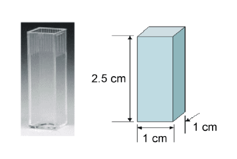
Figure 1: Shape and size of the polystyrene cuvette used in the computation.

The cuvette was exposed to a vertically polarized EM pulse the shape of which is described as a double exponential function (Samn and Mathur 1999)

$$E=E_{0}(e^{-\alpha t}-e^{-\beta t}).$$ (1)

$E_{0}$ is pulse amplitude and coefficients $\alpha$ and $\beta$ define the pulse rise time, fall time, and width. Numerical values of the parameters are roughly the ones measured in the GTEM cell used for bioelectromagnetic research at Louisiana Tech University: $E_{0}=18.5\;kV/m$, $\alpha=1.0\times 10^{8}\;s^{-1}$, and $\beta=2.0\times 10^{10}\;s^{-1}$. This pulse has a rise time of $\sim 150\;ps$ and a width of $\sim 10\;ns$. While detailed properties of a double exponential pulse can be found elsewhere (Dvorak and Dudley 1995), for better understanding of the results presented in this paper it is useful to know the frequency spectrum of the pulse used, which we plotted in Figure 2.

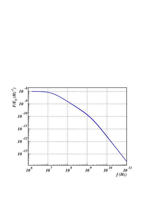
Figure 2: Frequency spectrum of the double exponential pulse, described in Equation 1, at the position of the source. $F/E_{0}$ denotes Fourier transform normalized to the field amplitude $E_{0}$.

The shape of the cuvette and the sample inside was discretized by means of Yee cells, cubes of edge length $\Delta x$. The Yee cells had to be small enough not to distort the shape and large enough for the time step, calculated from the Courant stability criterion (Taflove and Brodwin 1975, Kunz and Luebbers 1993, Taflove and Hagness 2000)

$$\Delta t\leq{1\over{c\sqrt{(\Delta x)^{-2}+(\Delta y)^{-2}+(\Delta z)^{-2}}}},$$ (2)

to be practical for overall computation. In Equation 2, in our case, $\Delta x=\Delta y=\Delta z$ and $c$ is the speed of light in vacuum. In order for the computation to be appropriate for the full frequency range of the EM pulse, the size of a Yee cell must also satisfy the rule

$$\Delta x\simeq{v\over{10\;f_{max}}},$$ (3)

where $v$ is the speed of light in the material and $f_{max}$ is the highest frequency considered defined by the pulse rise time

$$f_{r}={0.35\over\tau_{r}}.$$ (4)

In this equation $f_{r}$ is a maximum frequency in $Hz$ and $\tau_{r}$ is a rise time in $s$ (Faulkner 1969).

In the previous, as well as in the present work, the Yee cube edge length of $\Delta x=1/4\;mm$ satisfies all the above criteria and may be used to model blood exposure to the wave frequency of up to $15\;GHz$, a much greater value than required by the rise time criterion. The time step derived from the Courant criterion is $\Delta t\leq 0.48\;ps$. Optimal agreement between geometrical and physical descriptions eliminated the need for additional approximations and resulted in about one hour of computational time for every nanosecond of simulated time on a modern personal computer.

3 Dielectric Properties of Exposed Sample

Proper description of the dielectric properties of the exposed material is crucial when dealing with an UWB electromagnetic pulse. EM properties of a biological material are normally expressed in terms of frequency-dependent dielectric properties and conductivity, usually parametrized using the Cole-Cole model (Gabriel 1996, Gabriel et al 1996):

$$\varepsilon(\omega)=\varepsilon_{\infty}+\sum_{k=1}^{4}{\Delta\varepsilon_{k}\over{1+(i\omega\tau_{k})^{1-\alpha_{k}}}}+{\sigma\over i\omega\varepsilon_{0}},$$ (5)

where $i=\sqrt{-1}$, $\varepsilon_{\infty}$ is the permittivity in the terahertz frequency range, $\Delta\varepsilon_{k}$ are the drops in permittivity in a specified frequency range, $\tau_{k}$ are the relaxation times, $\sigma$ is the ionic conductivity, and $\alpha_{k}$ are the coefficients of the Cole-Cole model. They constitute up to 14 real parameters of a fitting procedure. While this function can be numerically Fourier transformed into the time domain, its application is problematic for FDTD. In addition to the physical problems arising when the Cole-Cole parametrization is applied (Simicevic and Haynie 2005), this parametrization requires time consuming numerical integration techniques and makes computation unacceptably slow.

If instead of a Cole-Cole parametrization one uses the Debye model in which the dielectric properties of a material are described as a sum of $N$ independent first-order processes

$$\varepsilon(\omega)=\varepsilon_{\infty}+\sum_{k=1}^{N}{\Delta\varepsilon_{k}\over{1+i\omega\tau_{k}}}=\varepsilon_{\infty}+\sum_{k=1}^{N}\chi_{k}(\omega),$$ (6)

then for each independent first-order process the Fourier transformation has an analytical solution

$$\chi_{k}(t)={\Delta\varepsilon_{k}\over\tau_{k}}\;e^{-t/\tau_{k}},\;\;{t\geq 0}.$$ (7)

$\chi(\tau)$ is the electric susceptibility of a material (Jackson 1999) and $\tau_{k}$ is the relaxation time for process $k$.

The static conductivity, $\sigma$, is defined in the time domain as the constant of proportionality between the current density and the applied electric field, $\vec{J}=\sigma\vec{E}$, and its implementation in FDTD does not require additional or different Fourier transforms (Kunz and Luebbers 1993).

The Debye parametrization allows use of a recursive convolution scheme (Luebbers et al 1990, 1991, Luebbers and Hunsberger 1992) and makes FDTD computation an order of magnitude faster compared to the use of numerical integration. In a recursive convolution scheme the permittivity at time step $(m+1)$ is simply the permittivity at time step $m$ multiplied by a constant (Kunz and Luebbers 1993). In addition to making the computation faster, in the previous work (Simicevic and Haynie 2005) we have shown that the Debye model also provides a sufficiently accurate description of physical properties of some biological materials. Here we use the same Debye parameters used in the previous two-dimensional calculation. The parameters applied in the Debye model of the form

$$\varepsilon(\omega)=\varepsilon_{\infty}+{{\varepsilon_{s1}-\varepsilon_{\infty}}\over{1+i\omega\tau_{1}}}+{{\varepsilon_{s2}-\varepsilon_{\infty}}\over{1+i\omega\tau_{2}}}$$ (8)

are shown in Table  1.

Material	$\varepsilon_{\infty}$	$\varepsilon_{s1}$	$\varepsilon_{s2}$	$\tau_{1}(s)$	$\tau_{2}(s)$	$\sigma(S/m)$
Polystyrene	2.0	-	-	-	-	0.
Water	4.9	80.1	-	$10.0\;10^{-12}$	-	0.
Blood	6.2	2506.2	65.2	$9.0\;10^{-8}$	$8.37\;10^{-12}$	0.7

Table 1: Debye parameters for the materials used in the computation (Simicevic and Haynie 2005).

4 Field Calculation and Data Representation

FDTD calculations of the exposure of a biological material to EM nanopulses provide the values of electric and magnetic field components at every space point and throughout the time range. In the case of a three-dimensional computation, there is overwhelming information such that data reduction and representation of the results becomes a nontrivial task. Contrary to radar applications where the interest is in scattered fields, here we care about total fields inside and closely sourrounding the sample. Even in such a restricted volume we have an immense number of data points and one has to carefully select the region of interest and the information to collect. The extraction of data depends on the physical model of interest and has to be decided prior to running the FDTD program.

The FDTD method enables easy creation of animated movies, which are very useful as a first step in the analysis and understanding of the behavior of the EM fields in space and time. The restriction of such visualization is that only parts of the full result can be represented at any given time and only in a chosen region of interest, typically in a few selected planes. As an example, snapshots of the penetration of an EM pulse into the cuvette, shown in Figure 1, filled with blood to the height of $2\;cm$ are shown in Figure 3. The complete animation can be accessed on-line (Simicevic 2005).

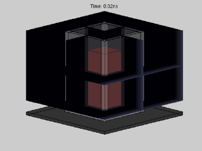
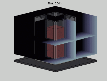
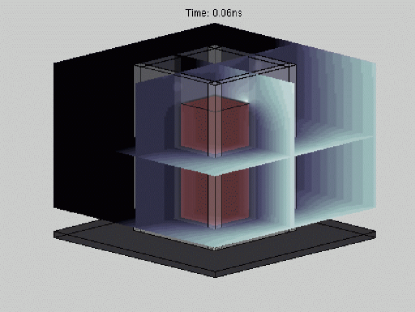
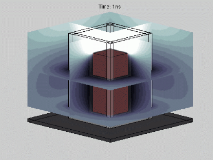
Figure 3: Penetration of an EM pulse into a blood-filled polystyrene cuvette. The contours represent the $z$-component of the electric field in steps of 1000 $V/m$. The dimension of the active area is $3\;cm$ $\times$ $3\;cm$ $\times$ $3\;cm$. Brighter regions correspond to a stronger field.

5 Results

In the previous two-dimensional calculation we have shown that the penetration of a linearly-polarized EM pulse described by Equation 1 into the blood-filled cuvette is governed by the pulse rise-time, creates a sub-nanosecond pulse, and is absorbed into a conductive loss of the material. While confirming the same results, the three-dimensional calculation also shows that the blood-filled cuvette behaves as a rectangular dielectric resonator.

In general, if a dielectric object is immersed in a incident sinusoidal wave, the EM fields in and around the object peak to high values at certain resonant frequencies. The object has a property of a resonator. The properties of dielectric resonators, such as resonant frequencies, field patterns, and quality factors, are difficult to obtain analytically except for a simple shapes such as, for example, a sphere (Van Bladel 1975). The FDTD method in combination with other techniques, like Fourier analysis or Prony’s method, can be used to determine the resonant frequencies and quality factors of dielectric resonators numerically (Navarro et al 1991, Harms et al 1992, Pereda et al 1992).

The resonant frequencies of a dielectric resonator depend on the size, shape and dielectric properties of the resonator (Kajfez and Guillon 1986). Generally, they can be found from the boundary condition at the surface between the resonator and the surrounding medium (Balanis 1989, Jackson 1999). In the case of a rectangular cavity resonator, a metal box, which can be filled with dielectric material, that traps the electromagnetic field, the resonant frequencies can be easily calculated using (Harrington 1961)

$$f_{mnp}={1\over{2\sqrt{\varepsilon\mu}}}\sqrt{\left({m\over a}\right)^{2}+\left({n\over b}\right)^{2}+\left({p\over c}\right)^{2}},$$ (9)

where $m=0,1,2,...\;$; $n=0,1,2,...\;$; $p=0,1,2,...\;$ are used as a label of the resonant mode. Also, $f_{mnp}$ is the corresponding resonant frequency, $\varepsilon$ and $\mu$ are the permittivity and permeability, respectively. The quantities a, b and c are the dimensions of the rectangular resonator.

For a pure dielectric box the situation is more complicated. The field is not entirely confined inside the box but it also exists as an evanescent wave outside the box. This wave decays exponentially with the distance from the dielectric. In our case, the complications arise also from the constant change of the exterior field caused by the incident pulse. The boundary conditions require that any tangential component of the electric field $\vec{E}$ be continuous, and that any normal component of electric displacement $\vec{D}$ be discontinuous by the amount of the charge density on the surface. Also, any normal component of the magnetic flux density $\vec{B}$ has to be continuous, and any tangential component of the magnetic field $\vec{H}$ has to be discontinuous by the amount of the surface current density. More detailed discussion of the boundary conditions and resonant modes of the dielectric resonator can be found in the paper by R. K. Mongia and A. Ittipiboon and references therein (Mongia and Ittipiboon 1997). Application of the boundary conditions in the FDTD calculation is discussed in more details by P. Yang et al (Yang et al 2004).

To find out what is happening when a dielectric box is immersed in the electromagnetic pulse, we have plotted the values of the x-component of the total field, $E_{x}$, for a selected time and in two planes: in the horizontal X-Y plane across the midpoint of the cuvette (left side of the Figure 4), and in the vertical X-Z plane across the same point (right side of the Figure 4). As a result of the boundary conditions, in both cases $E_{x}$ is discontinuous at the wall normal to its direction. At the wall parallel to the field direction, $E_{x}$ has to be continuous, but, since the outside field has to be continuous too, there is an abrupt change of the value of the $E_{x}$ component along the parallel wall, a change that is more prominent closer to the edges of the wall. While the details of the field behavior change from one time point to an other, the general feature stays the same. It is important to notice the formation of a resonant wave inside the dielectric on both sides of Figure 4.

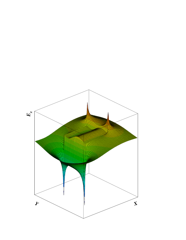
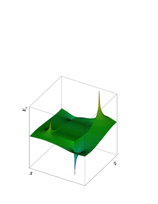
Figure 4: The $E_{x}$ component of the electric field inside and around the dielectric. Left: in the horizontal X-Y plane across the midpoint of the cuvette. Right: in the vertical X-Z plane across the same point. To understand the resonant behavior better, the cuvette walls were neglected in those pictures. The field values are taken 160 $ps$ after the pulse first impact on the dielectric.

It is not easy to estimate the resonant frequencies of a dielectric slab (Antar et al 1998). In the first approximation, assuming that the exponential decay of the evanescent wave with the distance from the slab is very fast, one can estimate the resonant frequency using Equation 9. We have calculated the lowest resonant frequency by selecting $m=n=p=1$, which allows for all the components of the EM field to exist. In our case $a=b=0.95\;cm$ and $c=2.0\;cm$. Since $\varepsilon$ in Equation 9 is a function of frequency described by the Debye model, the resonant frequency will be a function of frequency, too. If the dielectric resonator were immersed in the plane wave, we would expect the resonance to occur when the frequency of the wave is equal to the resonant frequency. In Figure 5 this corresponds to the intersection of the line $f_{111}=f$ and calculated resonant frequencies. For water the expected resonant frequency was found to be $f_{111}=2.66\;GHz$ and for blood $f_{111}=2.94\;GHz$. As shown in Figure 2, those frequencies are well inside the frequency spectrum of the double exponential pulse used in this calculation, therefore one can expect the resonant excitation to occur.

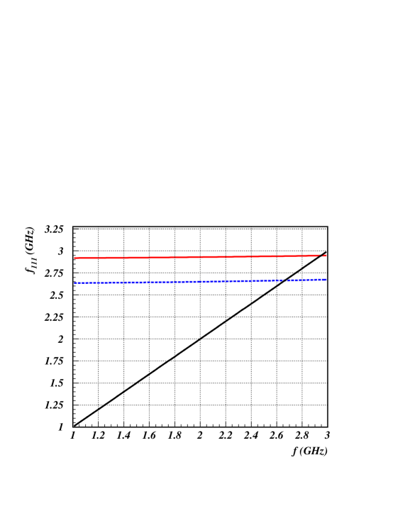
Figure 5: The resonant frequency as a function of frequency for blood (higher full red horizontal line) and water (lower dotted blue line). The resonant frequencies are shown only in the frequency region of interst. Intersections of the function $f_{111}=f$ with those lines are the expected resonant frequencies of the dielectric resonator.

To estimate the resonant frequencies using the FDTD data the field values were extracted at a fixed observation point inside the dielectric resonator as function of time. For any field component those values can be expressed in the form of free damped oscillator (Ko and Mittra 1991, Pereda et al 1992). Assuming just one resonant mode and selecting the $E_{x}$ component of the total field one can write

$$E_{x}(t)=Ae^{-\alpha t}\sin(2\pi f_{r}t)+B,$$ (10)

where $A$ is the modal amplitude, $\alpha$ is the damping factor, $f_{r}$ is the resonant frequency, and $B$ is small additional noise. The FDTD data fitted with this function are shown in Figure 6. The results of the fit are tabulated in Table  2. The ratio $B/A$ is less than 1%. Taking into consideration the simplicity of our model, the agreement between the expected resonant freqency and the one obtained through the fit is very good.

Knowing the resonant frequency and the damping factor, one can also obtain the quality factor $Q$ of the dielectric resonator using

$$Q=\pi f_{r}/\alpha.$$ (11)

The $Q$-factor is also tabulated in Table  2.

	$f_{r}$ (Eq. 9)	$f_{r}$ (Eq. 10)	$\alpha$	$Q$
Water	$2.66\;GHz$	$2.77\;GHz$	$2.35\;10^{9}\;s^{-1}$	$3.7$
Blood	$2.94\;GHz$	$2.49\;GHz$	$6.97\;10^{9}\;s^{-1}$	$1.1$

Table 2: Estimated and obtained resonant frequencies, damping factors and $Q$-factors for water and blood filled cuvette.

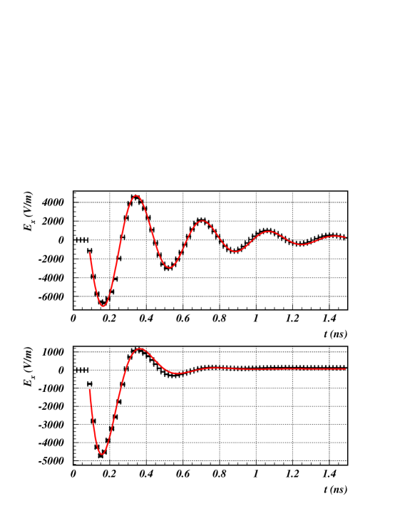
Figure 6: FDTD data at the cuvette’s mid point as a function of time. The upper histogram shows the data for water, and lower histogram for blood. The curves are the fits using Equation 10.

Finally, Figure 7 shows a few values of all the electric and magnetic field components in the blood and in the cuvette walls in the x-z plane during the pulse rise time. The curves are separated in time by 20 $ps$. As expected, the $E_{x}$, $E_{z}$, and $H_{y}$ are continuous and $E_{y}$, $H_{x}$, and $H_{z}$ are discontinuous at the boundaries of the materials. The buildup of a resonant steady wave is also shown.

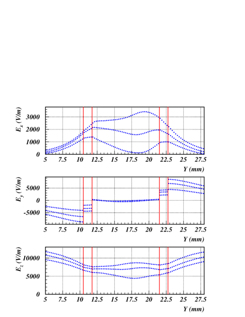
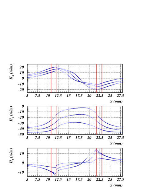
Figure 7: The values of all the electric and magnetic field components in the blood and in the cuvette walls, in the x-z plane, during the rise time of the pulse for three time periods separated by 20 $ps$.

The full three-dimensional computation of the exposure of the blood-filled cuvette to a linearly-polarized EM pulse described by Equation 1, not only reproduced the results of the two-dimensional computation, but also gave an insight into properties of induced components of the EM field. The three-dimensional calculation supports the notion that pulse penetration is a function of both rise time and pulse width, with both pulse features important in the case of a non-conductive material, right side of Figure 1, and the penetration dominated by rise time in the case of a conductive material, left side of Figure 1. It also shows that for a material of considerable conductivity, the incident pulse width is relatively unimportant. In addition, the three-dimensional calculation reveals that the dielectric box exposed to EM pulses behaves as a dielectric resonator.

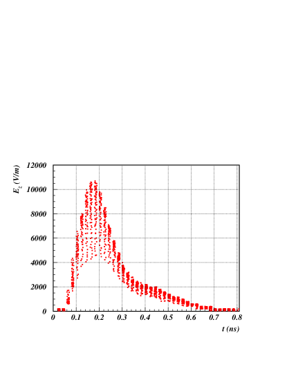
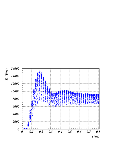
Figure 8: Left: the pulse shape of a blood-penetrated field component in the direction of pulse polarization for the first 0.8 $ns$. Right: the pulse shape of a water-penetrated field component in the direction of pulse polarization for the first 0.8 $ns$. Distribution of the field values in a particular time interval is a measure of the inhomogeneity of the field across the sample.

FDTD approach also allows calculation of the energy deposited in a biological material using (Jackson 1999)

$${{dE}\over{dt}}=\int_{V}\vec{J}\cdot\vec{E}\;dV\;=\;\sigma\;\int_{V}\vec{E}\cdot\vec{E}\;dV,$$ (12)

where ${dE}\over{dt}$ is the total energy per unit time absorbed in the volume, $\vec{J}$ and $\vec{E}$ are, respectively, the current density and electric field inside the material, and $\sigma$ is the conductivity of the material. FDTD computation provides all the above values through the entire time and it is easy to perform numerical integration of Equation 12. The results from the three-dimensional calculation are the same as from the two-dimensional calculation. For blood, the average converted energy per pulse, described by Equation 1, is again $\sim 0.003\;J/m^{3}$. The resulting temperature increase of $\sim 10^{-10}\;K$ per pulse is clearly negligible if the pulse repetition rate is low. Experiments performed by P. T. Vernier et al (Vernier et al 2004) have shown that even the nanopulses of similar duration but orders of magnitude higher field amplitude than the ones used in this work do not not cause significant intra- or extra-cellular Joule heating in the case of a low pulse repetition rate.

6 Conclusion

In this paper we have extended our previous FDTD calculations on nanopulse penetration into biological matter from two to three dimensions. Calculations included the same detailed geometrical description of the material exposed to nanopulses, the same accurate description of the physical properties of the material, the same spatial resolution of $1/4\;mm$ side length of the Yee cell, and the same cut-off frequency of $\sim 100\;GHz$ in vacuum and $\sim 15\;GHz$ in the dielectric. To minimize computation time, the dielectric properties of a tissue in the frequency range $\leq 100\;GHz$ were formulated in terms of the Debye parametrization which we have shown in a previous paper to be, for the materials studied, as accurate as the Cole-Cole parametrization.

The results of three-dimensional FDTD calculation can be summarized as follows:

a) The shape of a nanopulse inside a biomaterial is a function of both rise time and width of the incident pulse, with the importance of the rise time increasing as the conductivity of the material increases. Biological cells inside a conductive material are exposed to pulses which are often substantially shorter than the duration of the incident pulse. The same results followed from the two-dimensional calculation.

b) The dielectric material exposed to the EM pulse shows a behavior which can be attributed to the properties of a dielectric resonator. This result could not have been obtained by the two-dimensional calculation.

c) The amount of energy deposited by the pulse is small and no effect observed from exposure of a biological sample to nanopulses can have a thermal origin.

Calculation of the electric field surrounding a biological cell is a necessary step in understanding effects resulting from exposure to nanopulses. We have developed a complete FDTD code capable of this. In the near future, through the Louisiana Optical Network Initiative, we will have access to several supercomputers at Louisiana universities connected into one virtual statewide supercomputer. We will soon be able to calculate very complicated structures, larger size objects, and more complex materials.

References

References

- [1]
- [2] [] Antar Y M M, Cheng D, Seguin G, Henry B, and Keller M G 1998 Microwave and Optical Tech. Lett. 19 158
- [3] [] Balanis C A 1989 Advanced Engineering Electromagnetics New York: John Willey & Sons Inc.
- [4] [] Dvorak S L and Dudley D G 1995 IEEE Trans. Electomag. Compatibility 37 192
- [5] [] Faulkner E A 1969 Introduction to the Theory of Linear Systems London: Chapman and Hall
- [6] [] Federal Communications Commission 2002, News Release NRET0203, http://www.fcc.gov
- [7] [] Gabriel C 1996 Preprint AL/OE-TR-1996-0037, Armstrong Laboratory Brooks AFB, http://www.brooks.af.mil/AFRL/HED/hedr/reports/dielectric/home.html
- [8] [] Gabriel S, Lau R W and Gabriel C 1996 Phys. Med. Biol. 41 2251
- [9] [] Harrington R F 1961 Time-Harmonic Electromagnetic Fields New York: McGraw-Hill
- [10] [] Harms P H, Lee J F and Mittra R 1992 IEEE Trans. Microwave Theory Tech. MTT-40 741
- [11] [] Hu Q, Viswanadham S, Joshi R P, Schoenbach K H, Beebe S J and Blackmore P F 2005 Phys. Rev. E 71 031914
- [12] [] Jackson J D 1999 Classical Electrodynamics New York: John Willey & Sons Inc.
- [13] [] Kajfez D and Guillon P Eds. 1986 Dielectric Resonators MA: Artech House.
- [14] [] Ko W L and Mittra R 1991 IEEE Trans. Microwave Theory Tech. MTT-39 2176
- [15] [] Kunz K and Luebbers R 1993 The Finite Difference Time Domain Method for Electromagnetics Boca Raton: CRC Press LLC.
- [16] [] Luebbers R J, Hunsberger F, Kunz K S, Standler R B, and Schneider M 1990 IEEE Trans. Electromagn. Compat. 32 222
- [17] [] Luebbers R J, Hunsberger F, and Kunz K S 1991 IEEE Trans. Antennas Propagat. 39 29
- [18] [] Luebbers R J and Hunsberger F 1992 IEEE Trans. Antennas Propagat. 40 12
- [19] [] Miller R L, Murphy M R and Merritt J H 2002 Proceding of the 2nd International Workshop on Biological Effects of EMFs Rhodes Greece
- [20] [] Mongia R K and Ittipiboon A 1997 IEEE Trans. Antennas Propagat. AP-45 1348
- [21] [] Navarro A, Nuñez M J and Martin E 1991 IEEE Trans. Microwave Theory Tech. MTT-39 14
- [22] [] Pereda J A, Vielva L A, Vegas A and Prieto A 1992 IEEE Microwave Guided Wave Lett. 2 431
- [23] [] Polk C and Postow E eds. 1995 Handbook of Biological Effects of Electromagnetic Fields Boca Raton: CRC Press LLC.
- [24] [] Sadiku M N O 1992 Numerical Techniques in Electromagnetics Boca Raton: CRC Press LLC.
- [25] [] Samn S and Mathur S 1999 Preprint AFRL-HE-BR-TR-1999-0291, McKesson HBOC BioServices Brooks AFB.
- [26] [] Schoenbach K H, Joshi R P, Kolb J F, Chen N, Stacey M, Blackmore P F, Buescher E S, and Beebe S J 2004 Proceedings of the IEEE 92 1122
- [27] [] Simicevic N and Haynie D T 2005 Phys. Med. Biol. 50 347
- [28] [] Simicevic N 2005 http://caps.phys.latech.edu/neven/pulsefield/
- [29] [] Sullivan, D M 2000 Electromagnetic Simulation Using the FDTD Method New York: Institute of Electrical and Electronics Engineers.
- [30] [] Taflove A and Brodwin M E 1975IEEE Trans. on Microwave Theory and Techniques 23 623
- [31] [] Taflove A and Hagness S C 2000 Computational Electrodynamics: The Finite-Difference Time-Domain Method, 2nd ed. Norwood: Artech House.
- [32] [] Taylor J D ed. 1995 Introduction to Ultra-Wideband Radar Systems Boca Raton: CRC Press LLC.
- [33] [] Van Bladel J 1975 IEEE Trans. Microwave Theory Tech. MTT-23 199; Van Bladel J 1975 IEEE Trans. Microwave Theory Tech. MTT-23 208
- [34] [] Vernier P T, Sun Y, Marcu L, Craft C M and Gundersen M A 2004 Biophys. J. 86 4040
- [35] [] Yang P, Kattawar G W, Liou K-N and Lu J Q 2004 Applied Optics 43 4611
- [36] [] Yee K S 1966 IEEE Trans. Antennas Propagat. AP-14 302
- [37]