A sound card based multi-channel frequency measurement system

Abstract

For physical processes which express themselves as a frequency, for example magnetic field measurements using optically-pumped alkali-vapor magnetometers, the precise extraction of the frequency from the noisy signal is a classical problem. We describe herein a frequency measurement system based on an inexpensive commercially available computer sound card coupled with a software single-tone estimator which reaches Cramér–Rao limited performance, a feature which commercial frequency counters often lack. Characterization of the system and examples of its successful application to magnetometry are presented.

I Introduction

The present work is motivated by the need for a high resolution frequency measurement system for analyzing signals generated by optically-pumped cesium magnetometers Groeger et al. (2005a). A set of such magnetometers will be used for a detailed investigation of magnetic field fluctuations and gradients in an experiment searching for a neutron electric dipole moment (nEDM). The experiment calls for a magnetic field of between 1 to 2 $\mu\mbox{T}$ controlled at the 80 fT level when measured over 100 s time intervals, control corresponding to a relative uncertainty between 40 to 80 ppb. The magnetometers are based on the fact that for low magnetic fields the Larmor precession frequency $f_{L}$ in a vapor of Cs atoms is proportional to the modulus of the magnetic field $\vec{B}$

$$f_{L}=\gamma\left|\vec{B}\right|.$$ (1)

The proportionality factor $\gamma$ is a combination of fundamental and material constants and has a value of $\approx 3.5\>\mbox{kHz}/\mu\mbox{T}$ for ${}^{133}\mbox{Cs}$. The precession of the atoms modulates the resonant absorption coefficient of the cesium vapor, which is measured by a photodiode monitoring the power of a laser beam traversing the atomic vapor Bloom (1962). In the self-oscillating mode of operation Bloom (1962); Groeger et al. (2005b) the magnetometer signal is of the form

$$s(t)=A\sin{(2\pi f_{L}t+\phi)}+s_{0}\,.$$ (2)

The Larmor frequency, $f_{L}$, has to be extracted from the signal. Equation 1 connects the frequency determination precision directly to the resulting field measurement precision. The basic demand on the frequency measurement system in order to achieve the required field precision is a resolution of a few hundred $\mu\mbox{Hz}$ in an integration time of 100 s. Moreover, the synchronous detection of signals from an array of magnetometers requires a cost-effective multi-channel solution.

In our recent study Groeger et al. (2005b) of optically–pumped magnetometer performance, frequency measurements were made with a commercial frequency counter (Stanford Research Systems, model SR620), which has a limited frequency resolution, thereby limiting the magnetic field determination. Frequency counters rely on the detection of zero crossings of a periodic signal in a given dwell time. Their performance is limited by their resolution of the zero crossing times, an event which is affected by the amplitude, offset, and phase noise of the signal. In demanding applications, such as the one investigated here, that timing jitter limits the ultimate frequency resolution of the magnetometer signal measurement. Put simple, the limitation of frequency counters is due to the fact that they use only information in the vicinity of the zero crossings, while valuable wave form information from in between the zero crossings is ignored.

As a more powerful alternative one can use numerical frequency estimation algorithms to extract the frequency from the complete waveform sampled at an appropriate rate and with a sufficient resolution. The performance of an ADC-based measurement system for measuring a single frequency of about 8 Hz was discussed in Chibane et al. (1995). Under the assumption that a stable clock triggers the ADC, the authors in Chibane et al. (1995) show that the lower limit of the frequency resolution of their system coincides with the Cramér–Rao lower bound (CRLB) Kay (1993). The CRLB is a well-known concept from information theory and describes principle limits for the estimation of parameters from sampled signals.

In our application, the Larmor frequency in a magnetic field of $2\,\mu\mbox{T}$ lies in the audio frequency range ($f_{L}=7\,\mbox{kHz}$). We have investigated whether a commercially available (and rather inexpensive) professional multi-channel sound card would present a viable solution for sampling the magnetometer signals. The estimation of the frequency from the sampled data was done by a software algorithm. In the following we will show that such a simple system can indeed be used for CRLB limited real-time frequency measurements and for a detailed study of noise processes which limit the precision of atomic magnetometers.

II The system

The frequency measurement system consists of a professional sound card (M–Audio Delta 1010) for digitizing the analog input data, an atomic clock to provide a stable time reference, and a standard personal computer (PC) which reads the data and runs the frequency estimation algorithm. The sound card provides 8 analog input channels in a breakout box that connects to a PCI interface card in the PC. The analog input signals can be sampled with a resolution of up to 24 bit at a sampling rate of up to 96 kHz. In order to limit the amount of data we used only 16-bit resolution, which was proven to yield sufficient precision. Jitter or drifts of the sampling rate induce additional phase noise on the sampled signal which can seriously degrade the precision of the frequency estimation. An essential feature of the Delta 1010 sound card is its “world clock” input which can be used to phase-lock the internal clock of the sound card to an external 96 kHz time base. The time base was realized by a frequency generator synchronized to the 10 MHz signal of a rubidium frequency standard (Stanford Research Systems, model PRS10). The Rb frequency standard provides a relative stability of $10^{-12}$ in 100 s which minimizes possible sampling rate jitter and drifts far below the required level. The requirements for the PC system are not very demanding as long as it allows for the continuous recording of the 16 bit data sampled at a rate of 96 kHz (5.8 GB/h for 8 channels). A 1.8 GHz Pentium-4 processor was fast enough for real-time frequency determination for all eight channels at a given integration time. However, for the detailed analysis described below, in which the integration time is varied, the time series were evaluated off-line from the stored sampled data.

III Performance

Considering the magnetometer signal given by Eq. 2, the frequency $f_{L}$ is to be determined from the AC-coupled signal data which, after sampling, are of the form

$$x_{n}\! \!=\! \!\!A\sin{\left[2\pi\!\sum\limits_{k=1}^{n}\!\left(f_{L}+\delta f_{k}\right)\Delta t+\phi_{0}\!+\!\delta\phi_{n}\right]}\!+\delta x_{n},$$

$$n=(0,\ldots,N-1)\>,$$

where $A$ is the signal amplitude, $\Delta t$ the time resolution (inverse of the sampling rate $r_{s}$), and $\phi_{0}$ the initial phase. The number of sample points is $N=\tau/\Delta t\>(=\tau r_{s})$, where $\tau$ is the measurement integration time. Also shown is the noise contribution at each point $n$ arising from phase noise $\delta\phi_{n}$, frequency noise $\sum_{k=1}^{n}\delta f_{k}$, and offset noise $\delta x_{n}$. The frequency is determined from the data $x_{n}$ by a maximum likelihood estimator based on a numerical Fourier transformation which provides a CRLB limited value Rife and Boorstyn (1974). The algorithm iteratively searches for the frequency $f$ that maximizes the modulus of the Fourier sum

$$MF(f)=\left|\sum_{n=0}^{N-1}x_{n}W_{n}\exp\left({i\frac{2\pi f}{r_{s}}n}\right)\right|\>,$$ (4)

where $W_{n}$ is a windowing function.

Under ideal conditions (stable field and ideal electronics), the frequency and phase noise ($\delta f_{k}$ and $\delta\phi_{n}$) are not present in the signal (Eq. III). The fundamental noise contribution is the photocurrent shot noise, which is proportional to the square root of the DC offset $s_{0}$ in Eq. 2. The noise is converted, by a transimpedance amplifier, to voltage $V_{pc}$ and has a Gaussian amplitude distribution with zero mean, corresponding to a white frequency spectrum that is characterized by its power spectral density $\rho_{x}^{2}$ (in $\mbox{V}^{2}/\mbox{Hz}$). The signal-to-noise ratio (SNR) is defined as $A^{2}/(\rho_{x}^{2}f_{s})$, where $f_{s}=(2\Delta t)^{-1}=r_{s}/2$ is the sampling rate limited bandwidth, i.e., the Nyquist frequency or the highest frequency that can be detected unaliased. The CRLB of the frequency estimation from such an ideal magnetometer signal is given by the variance Kay (1993)

$$\sigma^{2}_{\mathrm{CRLB}}=\frac{3\rho_{x}^{2}}{\pi^{2}A^{2}\tau^{3}}.$$ (5)

noise source	$\sigma_{A}^{2}(\tau)$			$\sigma_{A}(\tau)$
white offset	$\displaystyle\frac{3}{\pi^{2}A^{2}}$$\cdot$	$\displaystyle\rho_{x}^{2}$ $\cdot$	$\displaystyle\frac{1}{\tau^{3}}$	$\propto\tau^{-3/2}$
flicker frequency	$\displaystyle 2\ln 2$$\cdot$	$\displaystyle h_{f}^{2}$ $\cdot$	$1$	$\propto\tau^{0}$
white frequency	$\displaystyle\frac{1}{2}$$\cdot$	$\displaystyle\rho_{f}^{2}$ $\cdot$	$\displaystyle\frac{1}{\tau}$	$\propto\tau^{-1/2}$
flicker phase	$\displaystyle\frac{3}{4\pi^{2}}$$\cdot$	$\displaystyle h_{\phi}^{2}$ $\cdot$	$\displaystyle\frac{\ln(2\pi f_{c}\tau)}{\tau^{2}}$	$\propto\tau^{-1}$
white phase	$\displaystyle\frac{3}{8\pi}$$\cdot$	$\displaystyle\rho_{\phi}^{2}$ $\cdot$	$\displaystyle\frac{f_{c}}{\tau^{2}}$	$\propto\tau^{-3/2}$

Table 1: The central column shows the dependence of the Allan variance $\sigma_{A}^{2}$ on the integration time $\tau$ and measurement bandwidth $f_{c}$ for the noise sources listed at the left Lesage and Audoin (1979). White noise sources $\alpha$ are characterized by their power spectral density $\rho^{2}_{\alpha}$. The frequency dependent spectral density of flicker noise process $\alpha$ is modeled by $\rho^{2}_{\alpha}(f)=h^{2}_{\alpha}/f$. By assuming the relation $f_{c}=(2\tau)^{-1}$ we find the power laws which typify each noise type, shown in the right hand column.

In frequency metrology it is customary to represent frequency fluctuations in terms of the Allan standard deviation $\sigma_{A}$ — or its square $\sigma_{A}^{2}$, the Allan variance Barnes et al. (1971); Lesage and Audoin (1979). One can show that for white noise $\sigma_{A}$ coincides with the classical standard deviation Allan (1987). A double logarithmic plot of the dependence of $\sigma_{A}$ on the integration time $\tau$ is a valuable tool for assigning the origin of the noise processes that limit the performance of an oscillator (see for example Barnes et al. (1971); Lesage and Audoin (1979)). As shown in Table 1, the variance $\sigma_{A}^{2}$ depends both on integration time $\tau$ and measurement bandwidth $f_{c}$, which, for a measurement interval $\tau$, is given by $f_{c}=(2\tau)^{-1}$. When that relation between bandwidth and integration time is inserted into the formulas given in the central column of Table 1 Lesage and Audoin (1979), one finds the typical $\tau$ dependencies of the Allan standard deviation $\sigma_{A}$ shown in the right-hand column. In the presence of several uncorrelated noise processes, $\alpha$, the variance of the estimated frequency is given by

$$\sigma^{2}=\sum\limits_{\alpha}\sigma^{2}_{\alpha}(f)\>.$$ (6)

Note that for a magnetometer signal, the contribution from Eq. 5 will always be present in the sum.

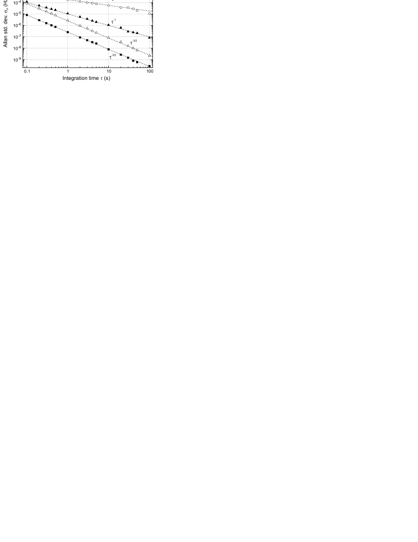
Figure 1: Allan standard deviation of the frequency of a synthesized sine wave affected by different noise processes. From top to bottom: flicker frequency noise (black dots), white frequency noise (open circles), flicker phase noise (black triangles), white phase noise (open triangles), white offset noise (black squares).

We first investigated whether our data analysis algorithm reproduces the theoretical $\tau$-dependencies shown in Table 1. For that purpose we generated time series (16 bit, 96 kHz) corresponding to Eq. III with only one of the phase, frequency, or offset noise terms enabled, and selected with well defined spectral characteristics (flicker or white). Figure 1 shows the Allan standard deviation $\sigma_{A}$ of those synthetic data. The emphasis here lies on the slopes rather than on the absolute values, which were chosen to yield a readable graph.

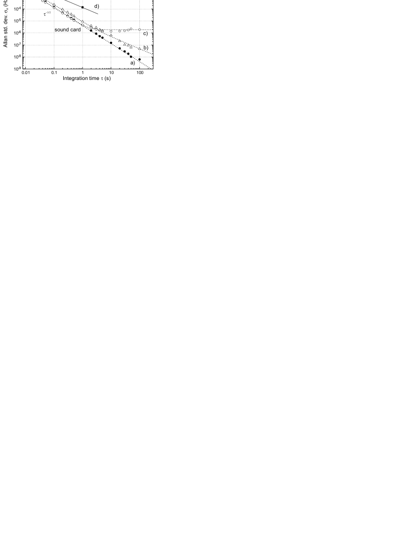
Figure 2: Allan standard deviation of the frequency of a sine wave affected by different noise processes, measured with the sound card (a–c) and a frequency counter (d): a) white offset noise, b) white offset noise and flicker phase noise, c) white offset noise and flicker frequency noise. The dashed lines represent the dependencies calculated on an absolute scale using the applied noise amplitudes. d) The same signal as in a) measured with a commercial frequency counter (Stanford Research model SR620) with a 300 Hz input bandpass filter.

Next, we investigated the ability of the sound card to reach CRLB limited detection of a 7 kHz sine wave. The wave was generated by a digital function generator (Agilent, model 33220A) stabilized to the same Rb frequency standard as the sound card. In order to simulate a signal comparable to that of the magnetometers, the SNR of the function generator output was artificially decreased from its nominal value of better than $5\times 10^{5}$ to about $1.3\times 10^{5}$ (in a 1 Hz bandwidth) by adding white offset noise. We recorded a 1 h time series of that signal, sampled with 16-bit resolution. The data were analyzed with the same algorithm as above and yielded an Allan standard deviation $\sigma_{A}(\tau)$, shown as black dots in Fig. 2a). The measurement agrees on an absolute scale with the CRLB calculated using Eq. 5 and the applied SNR. In addition to the offset noise, a second noise source was used to apply $1/f$ noise, in turn, to the frequency or to the phase modulation input of the function generator. The resulting $\sigma_{A}$ of the measured data is shown in Figs. 2b) and c). Figure 2d) shows $\sigma_{A}$ derived from the same signal as Fig. 2a) but analyzed by the commercial frequency counter (Stanford Research Systems, model SR620) that was used in Groeger et al. (2005b). The three points shown correspond to the three possible integration times of the SR620. It can be clearly seen that the counter technique does not allow the correct measurement of these faint noise processes. However, extrapolation of the data points suggest that for integration times less than 10 ms the CRLB could be reached.

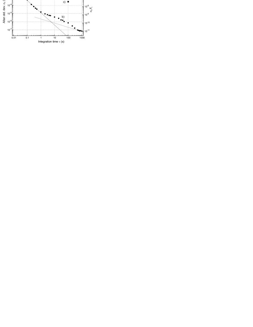
Figure 3: a) ASD $\sigma_{A}$ of magnetic field fluctuations inside a multi-layer magnetic shield. b) Residual fluctuations of the stabilized magnetic field. The dashed lines indicate the CRLB (left) and an assumed white frequency noise limitation (right). c) Stability required for the proposed nEDM experiment.

Finally, after the frequency estimator algorithm and the sound card had proven their CRLB performance limit, we used the system to analyze the frequency generated by an optically-pumped magnetometer (OPM). A magnetic field of $2\>\mu\mbox{T}$ was produced by a solenoid driven by an ultra-stable current source. The OPM signal in that field is a 7 kHz sine wave. The OPM and the solenoid were located in a 6-layer magnetic shield in order to suppress external field fluctuations. Figure 3a) shows $\sigma_{A}$ of a 2 h time series recorded with the sound card. The data represent pure magnetic field fluctuations. In particular, the approximately 2 mHz fluctuations in the range between 2 to 200 s could be traced back to irregular current fluctuations in the solenoid. Nevertheless, the relative field stability — and therefore the relative current stability — is on the order of $3\times 10^{-7}$ for that range of integration times. However, for a 100 s integration time the field instability exceeds the requirement for the nEDM experiment mentioned in the introduction.

In order to determine the magnetometer performance limit, we actively stabilized the magnetic field in the following way. The magnetometer frequency was compared to a stable reference oscillator (i.e., the Rb frequency standard) by means of a phase comparator, and the error signal was used to control the solenoid current, thus realizing a phase-locked loop. Figure 3b) shows the Allan standard deviation of the OPM in the stabilized field, which is CRLB-limited up to an integration time of 1 s. The noise excess between 1 and 300 s above the limits expected from the CRLB and the assumed white noise limitation shows the limitation of the current stabilization scheme, which nonetheless allows the suppression of the fluctuations by three orders of magnitude at the integration time of interest.

We have realized a frequency measurement system based on a digital sound card and have shown that it yields a performance superior to commercial frequency counters. We have proven that the system yields CRLB limited frequency resolution in measurements of sine waves affected by various sources of noise. We have used the system to prove that, at least in a limited range of integration times, an active field stabilization by an optically pumped magnetometer is limited by the theoretical Cramér-Rao bound. The performance and the multi-channel feature of the sound card and its external frequency reference option present a low-cost alternative for applications requiring simultaneous characterization of several frequency generation systems, especially for long integration times.

References

- Groeger et al. (2005a) S. Groeger, G. Bison, and A. Weis, To be published in: J. Res. Natl. Inst. Stand. Technol. 110(2005a).
- Bloom (1962) A. L. Bloom, Appl. Opt. 1, 61 (1962).
- Groeger et al. (2005b) S. Groeger, A. S. Pazgalev, and A. Weis, Appl. Phys. B 80, 645 (2005b).
- Chibane et al. (1995) Y. Chibane, S. K. Lamoreaux, J. M. Pendlebury, and K. F. Smith, Meas. Sci. Technol. 6, 1671 (1995).
- Kay (1993) S. M. Kay, Fundamentals of Statistical Signal Processing, Volume I: Estimation Theory, Prentice-Hall signal processing series (Prentice Hall PTR, Upper Saddle River, New Jersey 07458, 1993).
- Rife and Boorstyn (1974) D. C. Rife and R. R. Boorstyn, IEEE Trans. Inf. Theory 20, 591 (1974).
- Barnes et al. (1971) J. Barnes, A. R. Chi, L. Cutler, D. Healey, D. Leeson, T. McGunigal, J. Mullen, Jr., W. Smith, R. Sydnor, et al., IEEE Trans. Instrum. Meas. 20, 105 (1971).
- Lesage and Audoin (1979) P. Lesage and C. Audoin, Radio Science 14, 521 (1979).
- Allan (1987) D. W. Allan, IEEE Trans. Ultrason. Ferroel. Freq. Contr. 34, 647 (1987).