Simultaneous cooling of axial vibrational modes in a linear ion-trap

Abstract

In order to use a collection of trapped ions for experiments where a well defined preparation of vibrational states is necessary, all vibrational modes have to be cooled to ensure precise and repeatable manipulation of the ions’ quantum states. A method for simultaneous sideband cooling of all axial vibrational modes is proposed. By application of a magnetic field gradient the absorption spectrum of each ion is modified such that sideband resonances of different vibrational modes coincide. The ion string is then irradiated with monochromatic electromagnetic radiation, in the optical or microwave regime, for sideband excitation. This cooling scheme is investigated in detailed numerical studies. Its application for initializing ion strings for quantum information processing is extensively discussed.

I Introduction

Atomic ions trapped in an electrodynamic cage allow for preparation and measurement of individual quantum systems, and represent an ideal system to investigate fundamental questions of quantum physics, for instance, related to decoherence Myatt00 ; Roos99 , the measurement process Hannemann02 ; Wunderlich03 , or multiparticle entanglement Entangle . Also, trapped ions satisfy all criteria necessary for quantum computing. Two internal states of each ion represent one elementary quantum mechanical unit of information (a qubit). The quantized vibrational motion of the ions (the “bus-qubit”) is used as means of communication between individual qubits to implement conditional quantum dynamics with two or more qubits Cirac95 . In recent experiments quantum logic operations with two trapped ions were realized QGate and teleportation of an atomic state has been demonstrated Teleport .

These implementations of quantum information processing (QIP) with trapped ions require that the ion string is cooled to low vibrational collective excitations Cirac95 ; QGate ; Sorensen00 ; Jonathan00 . In particular, this condition should be fulfilled by all collective vibrational modes Wineland98 . Therefore, in view of the issue of scalable QIP with ion traps, it is important to find efficient cooling schemes that allow to prepare vibrationally cold ion chains.

Cooling of the vibrational motion of two ions in a common trap potential has been demonstrated experimentally King98 ; Peik99 ; Roos00 ; Reiss02 (see also Eschner03 for a recent review). This is deemed to be sufficient for a quantum information processor which utilizes two ions at a time for quantum logic operations with additional ions stored in spatially separated regions Kielpinski02 . If more than two ions reside in a common trap potential and shall be used simultaneously for quantum logic operations, however, the task of reducing the ions’ motional thermal excitation becomes increasingly challenging with a growing number of ions and represents a severe obstacle on the way towards scalable QIP with an ion chain. Straightforward extensions of laser-cooling schemes for one particle to many ions, like sequentially applying sideband cooling Eschner03 to each one of the modes, becomes inefficient as the number of ions increases, since after having cooled the last mode, the first one may already be considerably affected by heating due to photon scattering and/or due to fluctuations of the trap potential. Therefore, it is desirable to find a method that allows for simultaneous and efficient cooling of many vibrational modes of a chain of ions.

In this article we propose a scheme that allows for simultaneous sideband cooling of all collective modes of an ion chain to the ground state. This is achieved by inducing position dependent Zeeman shifts through a suitably designed magnetic field, thereby shifting the spectrum of each ion in such a way that the red-sideband transitions of each mode may occur at the same frequency. Thus, by irradiating the ion string with monochromatic radiation all axial modes are cooled. We investigate numerically the efficiency and explore implementations of simultaneous sideband excitation by means of laser light, and alternatively, by using long-wavelength radiation in the radio-frequency or microwave regime Mintert01 ; Wunderlich02 ; McHugh05 .

The remainder of this article is organized as follows: In section II the cooling scheme is outlined. Numerical investigations of the cooling efficiency are presented for implementations using an optical Raman transition (section III) and a microwave transition (section IV). In section V possible experimental implementations are discussed and the cooling scheme is studied under imperfect experimental conditions. The paper is concluded in section VI.

II The concept of simultaneous sideband cooling

II.1 Axial vibrational modes

We consider $N$ crystallized ions each of mass $m$ and charge $e$ in a harmonic trap. The trap potential has cylindrical symmetry around the $z-$axis providing strong radial confinement such that the ions are aligned along this axis Footnote:Example . We denote by $\nu_{r}$, $\nu_{z}$ the radial and axial frequencies of the resulting harmonic potential, where $\nu_{r}\gg\nu_{z}$, and by $z_{j}^{(0)}$ the ions classical equilibrium positions along the trap axis. The typical axial distance $\delta z$ between neighboring ions scales like $\delta z\sim\zeta_{0}2N^{-0.57}$ with $\zeta_{0}\equiv(e^{2}/(4\pi\epsilon_{0}m\nu_{1}^{2}))^{1/3}$Steane97 ; James98 . For brevity, in the remainder of this article, the ion at the classical equilibrium position $z_{j}^{(0)}$ is often referred to as ”ion $j$”.

At sufficiently low temperatures the ions vibrations around their respective equilibrium positions are harmonic and the axial motion is described by $N$ harmonic oscillators according to the Hamiltonian

$$\tilde{H}_{\rm mec}=\sum_{\alpha=1}^{N}\hbar\nu_{\alpha}(a_{\alpha}^{\dagger}a_{\alpha}+1/2)\ ,$$ (1)

where $\nu_{\alpha}$ are the frequencies of the chain collective modes and $a_{\alpha}^{\dagger}$ and $a_{\alpha}$ the creation and annihilation operators of a phonon at energy $\hbar\nu_{\alpha}$. We denote with $Q_{\alpha},P_{\alpha}$ the corresponding quadratures, such that $[Q_{\alpha},P_{\alpha}]={\rm i}\hbar$, and choose the labelling convention $\nu_{1}<\nu_{2}<\ldots<\nu_{N}$, whereby $\nu_{1}=\nu_{z}$ (in this article we often refer to the collective vibrational mode characterized by $\nu_{\alpha}$ as ”mode $\alpha$”). The local displacement $q_{j}=z_{j}-z_{j}^{(0)}$ of the ion $j$ from equilibrium is related to the coordinates $Q_{\alpha}$ by the transformation

$$q_{j}=\sum_{\alpha}S_{j}^{\alpha}Q_{\alpha}$$ (2)

where $S_{j}^{\alpha}$ are the elements of the unitary matrix $S$ that transforms the dynamical matrix $A$, characterizing the ions potential, such that $S^{-1}AS$ is diagonal. The frequencies, $\nu_{\alpha}$ of the vibrational modes are given by $\sqrt{\upsilon_{\alpha}}\times\nu_{1}$ where $\upsilon_{\alpha}$ are the eigenvalues of $A$ James98 . The normal modes are excited by displacing an ion from its equilibrium position $z_{j}^{(0)}$ by an amount $q_{j}$. Thus, the coefficients $S_{j}^{\alpha}$ describe the strength with which a displacement $q_{j}$ from $z_{j}^{(0)}$ couples to the collective mode $\alpha$.

Excitation of a vibrational mode can be achieved through the mechanical recoil associated with the scattering of photons by the ions. This excitation is scaled by the Lamb-Dicke parameter (LDP) Stenholm86 , which for a single ion corresponds to $\sqrt{\omega_{R}/\nu}$, where $\omega_{R}=\hbar k^{2}/2m$ is the recoil frequency and $\hbar k$ the linear momentum of a photon. In an ion chain we associate a Lamb-Dicke parameter $\eta_{\alpha}$ with each mode according to the equation

$$\eta_{\alpha}=\sqrt{\frac{\omega_{R}}{\nu_{\alpha}}}\ .$$ (3)

Hence, if a photon is scattered by the ion at $z_{j}^{(0)}$, the ion recoil couples to the mode $\alpha$ according to the relation Morigi01

$$\eta_{j}^{\alpha}=S_{j}^{\alpha}\eta_{\alpha}\ .$$ (4)

In the remainder of this article we will assume that the ions are in the Lamb-Dicke regime, corresponding to the fulfillment of condition $\sqrt{\langle a_{\alpha}^{\dagger}a_{\alpha}\rangle}\eta_{\alpha}\ll 1$. In this regime the scattering of a photon does not couple to the vibrational excitations at leading order in this small parameter, while changes of one vibrational quantum $\hbar\nu_{\alpha}$ occur with probability that scales as $|\eta_{\alpha}|^{2}$. Changes by more than one vibrational quantum are of higher order and are neglected here.

II.2 Sideband cooling of an ion chain

In this section we consider a schematic description of sideband cooling of an ion chain, in order to introduce the concepts relevant for the following discussion. We denote by $|0\rangle$ and $|1\rangle$ the internal states of the ion transition at frequency $\omega_{0}$, in absence of external fields, and linewidth $\gamma$. A spatially inhomogeneous magnetic field is applied that shifts the transition frequency of each ion individually such that for the ion at position $z_{j}^{(0)}$ the value $\omega_{j}$ is assumed. Each ion transition couples to radiation at frequency $\omega_{L}$, which drives it well below saturation. In this limit, the contributions of scattering from each ion to the excitation of the modes add up incoherently Morigi99 ; Morigi01 .

For this system, the equations describing the dynamics of laser sideband cooling of an ion chain can be reduced to rate equations of the form

$$\frac{\rm d}{{\rm d}t}P_{\alpha}(n^{(\alpha)}) = (n^{(\alpha)}+1)\left[A_{-}^{\alpha}P_{\alpha}(n^{(\alpha)}+1)-A_{+}^{\alpha}P_{\alpha}(n^{(\alpha)})\right]$$ (5)

$$-n^{(\alpha)}\left[A_{-}^{\alpha}P_{\alpha}(n^{(\alpha)})-A_{+}^{\alpha}P_{\alpha}(n^{(\alpha)}-1)\right]$$

where $P_{\alpha}(n^{(\alpha)})$ is the average occupation of the vibrational number state $|n^{(\alpha)}\rangle$ of the mode $\alpha$, and $A_{+}^{\alpha}$ ($A_{-}^{\alpha}$) characterizes the rate at which the mode is heated (cooled). Equation (5) is valid in the Lamb-Dicke regime, i.e. when the LDP is sufficiently small to allow for a perturbative expansion in this parameter. Denoting by $\Omega_{j}$ the Rabi frequency, the heating and cooling rate takes the form Morigi01

$$A_{\pm}^{\alpha}=\sum_{j=1}^{N}|\eta_{j}^{\alpha}|^{2}\frac{\Omega_{j}^{2}}{2\gamma}\left[\frac{\gamma^{2}}{4(\delta_{j}\mp\nu_{\alpha})^{2}+\gamma^{2}}+\phi\frac{\gamma^{2}}{4\nu_{\alpha}^{2}+\gamma^{2}}\right]$$ (6)

where the detuning $\delta_{j}\equiv\omega_{L}-\omega_{j}$. The coefficient $\phi$ emerges from the integral over the angles of photon emission, according to the pattern of emission of the given transition Stenholm86 . For $A_{-}^{\alpha}>A_{+}^{\alpha}$ a steady state exists, it is approached at the rate

$$\Gamma_{\rm cool}^{(\alpha)}=A_{-}^{\alpha}-A_{+}^{\alpha}$$ (7)

and the average number of phonons of mode $\alpha$ at steady state is given by the expression

$$\langle n^{(\alpha)}\rangle=\frac{A_{+}^{\alpha}}{A_{-}^{\alpha}-A_{+}^{\alpha}}\ .$$ (8)

Sideband cooling reaches $\langle n^{(\alpha)}\rangle\ll 1$ through $A_{-}^{\alpha}\gg A_{+}^{\alpha}$. This condition is obtained by selectively addressing the motional resonance at $\omega_{0}-\nu_{\alpha}$. This is accomplished for a single collective mode when $\gamma\ll\nu_{\alpha}$ and $\delta_{\alpha}=\nu_{\alpha}$.

In this work, we show how the application of a suitable magnetic field allows for simultaneous sideband cooling of all modes. In particular, the field induces space-dependent frequency shifts that suitably shape the excitation spectrum of the ions. Simultaneous cooling is then achieved when for each mode $\alpha$ there is one ion $j$ with the matching resonance frequency, that is, such that $\delta_{j}=\omega_{L}-\omega_{j}=\nu_{\alpha}$. This procedure is outlined in detail in the following subsection.

II.3 Shaping the spectrum of an $N$ ion chain

Assume the ion transition $|0\rangle\to|1\rangle$ and that a magnetic field–whose magnitude varies as a function of $z$–is applied to the linear ion trap, Zeeman shifting this resonance. As a result, the ions resonance frequencies $\omega_{j}$ are no longer degenerate. The field gradient is designed such that all ions share a common motion-induced resonance. This resonance corresponds to one of the transitions $|0,n^{(\alpha)}\rangle\to|1,n^{(\alpha)}-1\rangle$, namely to the red sideband of the modes $\alpha$. The resonance frequency of each ion is shifted such that the red sidebands of all modes can be resonantly and simultaneously driven by monochromatic radiation at frequency $\omega=\omega_{1}-\nu_{1}=\ldots=\omega_{N}-\nu_{N}$. Ionic resonances and the associated red sideband resonances–optimally shifted for simultaneous cooling–are illustrated in Fig. 1 for the case of 10 ions.

Sideband excitation can be accomplished by either laser light or microwave radiation according to the scheme discussed in Mintert01 . With appropriate recycling schemes this leads to sideband cooling on all $N$ modes simultaneously. A discussion on how a suitable field gradient shifting the ionic resonances in the desired fashion can be generated is deferred to section V.

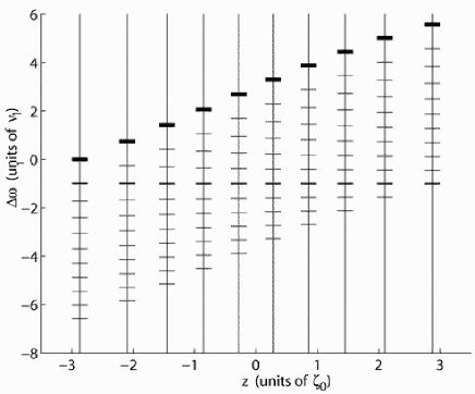
Figure 1: Illustration of the axial motional spectrum of a chain of 10 ions in the presence of a spatially inhomogeneous magnetic field. The vertical lines indicate the axial position of each ion in units of $\zeta_{0}$. The corresponding horizontal lines indicate the frequencies of the spectral lines as measured at that particular ion. The thick horizontal lines indicate the ions resonance frequencies $\omega_{j}-\omega_{1}$ (in units of the secular axial frequency $\nu_{1}$) relative to the resonance frequency $\omega_{1}$ of the ion at $z_{1}=-2.87\zeta_{0}$. The remaining horizontal lines show the frequencies of red sideband resonances for each ion at frequencies $\omega_{j}-\nu_{\alpha}$ ($j,\alpha=1,\ldots,10$). The magnetic field is designed such that $\omega_{1}-\nu_{1}=\omega_{2}-\nu_{2}=\ldots\omega_{N}-\nu_{N}$. These resonances are highlighted by medium thick lines.

II.4 Theoretical model

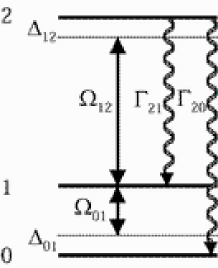
Figure 2: Schematic of the ions internal energy levels on which cooling is implemented. Indicated are the relevant Rabi frequencies (symbols $\Omega$), spontaneous decay rates ($\Gamma$), and detunings ($\Delta$). The corresponding equations for the dynamics are discussed in detail in the appendix

As an example, we discuss simultaneous sideband cooling of the collective axial modes of a chain composed of ¹⁷¹Yb⁺ions with mass $m=171$ a.m.u.. The ions are crystallized along the axis of a linear trap characterized by $\nu_{1}=1\times 2\pi$MHz. A magnetic field $B(z)$ along the axis is applied that Zeeman-shifts the energy of the internal states. The value of the field along $z$ is such that it shifts the red-sidebands of all modes into resonance along the chain, while at the same time its gradient is sufficiently weak to negligibly affect the frequencies of the normal modes Wunderlich02 .

The selective drive of the motional sidebands can be implemented on a magnetic dipole transition in ¹⁷¹Yb⁺close to $\omega_{0}=12.6\times 2\pi$ GHz between the hyperfine states $|0\rangle=|S_{1/2},F=0\rangle$ and $|1\rangle=|S_{1/2},F=1,m_{F}=1\rangle$. The magnetic field gradient lifts the degeneracy between the resonances of individual ions, and the transition frequency $\omega_{j}$ of ion $j$ is proportional to $B(z_{j})$ in the weak field limit $\mu_{B}B/\hbar\omega_{0}\ll 1$, where $\mu_{B}$ is the Bohr magneton. For strong magnetic fields the variation of $\omega_{j}$ with $B$ is obtained from the Breit-Rabi formula Wunderlich03 .

We investigate two cases, corresponding to two different implementations of the excitation of the sideband transition between states $|0\rangle$ and $|1\rangle$. In the first case, discussed in section III, the sideband transition is driven by two lasers with appropriate detuning, namely a Raman transition is implemented with intermediate state $|2\rangle=|P_{1/2}\rangle$. In the second case, presented in section IV, microwave radiation drives the magnetic dipole.

Since spontaneous decay from state $|1\rangle$ back to $|0\rangle$ is negligible on this hyperfine transition, laser light is used to optically pump the ion into the $|0\rangle$ state via excitation of the $|1\rangle\to|2\rangle$ electric dipole transition. This laser light is close to 369nm and serves at the same time for state selective detection by collecting resonance fluorescence on this transition, and for initial Doppler cooling of the ions. The state $|2\rangle$ decays with rates $\Gamma_{21}=11\times 2\pi$MHz and $\Gamma_{20}=5.5\times 2\pi$MHz into the states $|1\rangle$ and $|0\rangle$, respectively FootnoteB . The considered level scheme is illustrated in Fig. 2, and the corresponding model is described in the appendix.

We evaluate the efficiency of the cooling procedure by neglecting the coupling between different vibrational modes by photon scattering, which is reasonable when the system is in the Lamb-Dicke regime. In this case, the dynamics reduce to solving the equations for each mode $\alpha$ independently, and the contributions from each ion to the dynamics of the mode are summed up incoherently Morigi01 , as outlined in Sec. II.2. The steady state and cooling rates for each mode are evaluated using the method discussed in Marzoli94 and extended to a chain of $N$ ions. The extension of this method to a chain of ions is presented in the appendix. The numerical calculations were carried out for this scheme and chains of $N$ ions with $1<N\leq 10$ and for some values $N>10$. Since the qualitative conclusions drawn from these calculations did not depend on $N$, we therefore restrict the discussion in sections III, IV, and V to the case $N=10$.

III Raman sideband cooling of an ion chain

We consider sideband cooling of an ion chain when the red sideband transition is driven by a pair of counter-propagating lasers, which couple resonantly the levels $|0\rangle$ and $|1\rangle$. The two counter-propagating light fields couple with frequency $\omega_{R1}$, $\omega_{R2}$ to the optical dipole transitions $|0\rangle\to|2\rangle$ and $|1\rangle\to|2\rangle$, respectively. The two lasers are far detuned from the resonance with level $|2\rangle$ such that spontaneous Raman transitions are negligible compared to the stimulated process. We denote by $\Delta_{01}=[(\omega_{R1}-\omega_{R2})-\omega_{1}]$ the Raman detuning, such that $\Delta_{01}=0$ corresponds to driving resonantly the transition $|0\rangle\to|1\rangle$ at the first ion in the chain, and by $\Omega_{01}$ the Rabi frequency describing the effective coupling between the two states. A third light field with Rabi frequency $\Omega_{12}$ is tuned close to the resonance $|1\rangle\to|2\rangle$ and serves as repumper into state $|0\rangle$ (compare Fig. 2). The frequencies $\omega_{Ri}$ are close to the ¹⁷¹Yb⁺resonance at 369nm, and the trap frequency is $\nu=1\times 2\pi$MHz. Hence, from Eq. (3) the Lamb-Dicke parameter takes the value $\eta_{1}\approx 0.0926$.

III.1 Sequential cooling

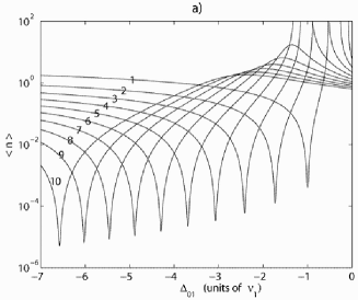
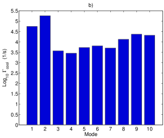
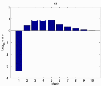
Figure 3: Raman sideband cooling of a chain of 10 ions without magnetic field gradient. The parameters are $\Omega_{12}=100\times 2\pi$kHz, $\Omega_{01}=30\times 2\pi$kHz, $\Delta_{12}=-10\times 2\pi$MHz. a) Steady state mean vibrational number $\langle n^{(\alpha)}\rangle$ as a function of $\Delta_{01}$ in units of $\nu_{1}$. b) Cooling rate $\Gamma_{\rm cool}^{(\alpha)}$ of mode $\alpha$ for $\Delta_{01}=-\nu_{\alpha}$. c) Steady state populations for $\Delta_{01}=-\nu_{1}$, corresponding to sideband cooling of mode 1. The bars indicating the vibrational excitations of modes $\nu_{3}$ and $\nu_{4}$ have been truncated.

In absence of external field gradients shifting inhomogeneously the ions transition frequencies (namely, when $\omega_{1}=\ldots=\omega_{N}=\omega_{0}$), cooling of an ion chain could be achieved by applying sideband cooling to each mode sequentially. In each step of the sequence all ions are illuminated simultaneously by laser light with detuning $\Delta_{01}=-\nu_{\alpha}$, thereby achieving sideband cooling of a particular mode $\alpha$. Since all ions are illuminated, they all contribute to the cooling of mode $\alpha$.

In Fig. 3a) the steady state vibrational number of each mode at the end of the cooling dynamics is displayed as a function of the relative detuning $\Delta_{01}$. Each mode $\nu_{\alpha}$ reaches its minimal excitation at values of the detuning $\Delta_{01}=-\nu_{\alpha}$. Therefore, in order to cool all modes close to their ground state, the detuning of the laser light has to be sequentially set to the optimal value for each mode $\alpha$.

The cooling rates $\Gamma^{(\alpha)}_{\rm cool}$ of mode $\alpha$ at $\Delta_{01}=-\nu_{\alpha}$, as defined in Eq. (7), are displayed in Fig. 3b). They are different for each mode and vary between 1kHz and 100kHz for the parameters chosen here. Even though these cooling rates would, in principle, allow for cooling sequentially all modes in a reasonably short time, this scheme may not be effective, since while a particular mode $\alpha$ is cooled all other modes are heated (i) by photon recoil, and, (ii) by coupling to the environment. As external source of heating we consider here the coupling of the ions charges to the fluctuating patch fields at the electrodes Turchette00 . The effects of these processes on the efficiency of cooling are discussed in what follows.

The consequences of heating due to photon scattering are visible in Fig. 3a). Here, one can see that while cooling one mode, others can be simultaneously heated, such that their average phonon number at steady state is very large. These dynamics are due to the form of the resonances in a three-level configuration Marzoli94 ; EIT00 . In general, however, the time scale of heating processes due to photon scattering is considerably longer than the time scale at which a certain mode is optimally sideband cooled, since the transitions leading to heating are out of resonance. In the case discussed in Fig. 3, for instance, the heating rates of these modes at $\Delta_{01}=-\nu_{1}$ are orders of magnitude smaller than the cooling rate of mode 1, and their dynamics can be thus neglected while mode 1 is sideband cooled. Similar dynamics are found for $\Delta_{01}=-\nu_{\alpha}$. Thus, in general one may neglect photon scattering as source of unwanted heating of modes that are not being efficiently cooled.

Nevertheless, heating by fluctuating electric fields occurs with appreciable rates ranging between 5s^-1 and $10^{4}$s^-1 Turchette00 . The heating rate is different for each mode and was observed to be considerably larger for the COM mode (here denoted as mode 1) than for modes that involve differential relative displacements of individual ions. Obviously, cooling can only be achieved, if the cooling rate $\Gamma_{\rm cool,seq}^{(\alpha)}$ of each mode exceeds in magnitude the corresponding trap heating rate denoted by $\Gamma_{\rm heat}^{(\alpha)}$:

$$\Gamma_{\rm heat}^{(\alpha)}\ll\Gamma_{\rm cool,seq}^{(\alpha)}\forall\alpha=1,\ldots,10\ .$$ (9)

In addition, one must consider that after a particular mode $\alpha$ has been cooled, it might heat up again while all other modes, $\beta\neq\alpha$ are being cooled. This imposes a second condition on the cooling rate. In order to quantify this second condition, we first evaluate the time, $T_{\rm cool}^{(\alpha)}$ it takes to cool one particular mode $\alpha$ from an initial thermal distribution, obtained by means of Doppler cooling and characterized by the average occupation number $\langle n^{(\alpha)}\rangle_{i}$, to a final distribution characterized by $\langle n^{(\alpha)}\rangle_{f}$. This time can be estimated to be Stenholm86

$$T_{\rm cool}^{(\alpha)}\equiv\ln\frac{\langle n^{(\alpha)}\rangle_{i}}{\langle n^{(\alpha)}\rangle_{f}}/(\Gamma_{\rm cool,seq}^{(\alpha)}-\Gamma_{\rm heat}^{(\alpha)})\ .$$ (10)

where $\langle n^{(\alpha)}\rangle_{f}\ll 1$ at steady state was assumed.

From this relation one obtains the total time, $T_{\rm seq}^{(\alpha)}$ needed to cool all modes except mode $\alpha$, or, in other words the time during which mode $\alpha$ is not cooled and could get heated. This time, $T_{\rm seq}^{(\alpha)}$ needed to sideband cool all modes with $\beta\neq\alpha$ is

$$T_{\rm seq}^{(\alpha)}=\sum_{\beta,\beta\neq\alpha}T_{\rm cool}^{(\beta)}=\sum_{\beta\neq\alpha}\ln\frac{\langle n^{(\beta)}\rangle_{i}}{\langle n^{(\beta)}\rangle_{f}}1/(\Gamma_{\rm cool,seq}^{(\beta)}-\Gamma_{\rm heat}^{(\beta)})\ .$$ (11)

If mode $\alpha$ is to stay cold during this time, the heating rate affecting it must be small enough. Hence the condition for efficient sequential sideband cooling is derived,

$$\Gamma_{\rm heat}^{(\alpha)}\times T_{\rm seq}^{(\alpha)}\ll 1$$ (12)

namely, during time $T_{\rm seq}^{(\alpha)}$, necessary for cooling the modes $\beta\neq\alpha$, the heating of mode $\alpha$ has to be negligible. Clearly, this condition is stronger than the one derived in relation (9), and its fulfillment becomes critical as the number of vibrational modes (ions) is increased.

A rough estimate of the time $T_{\rm seq}^{(\alpha)}$ to be inserted in (12) can be obtained from eq. (11) under the assumption that all modes start out with the same mean excitation $\langle n\rangle_{i}$ (usually determined by initial Doppler cooling) and are cooled to the same final excitation $\langle n\rangle_{f}$. Using condition (9), one obtains

$$T_{\rm seq}^{(\alpha)}\approx\ln\frac{\langle n\rangle_{i}}{\langle n\rangle_{f}}\sum_{\beta\neq\alpha}1/\Gamma_{\rm cool,seq}^{(\beta)}\ .$$ (13)

Substituting this expression into (12) gives

$$\Gamma_{\rm heat}^{(\alpha)}\ll\left(\ln\frac{\langle n\rangle_{i}}{\langle n\rangle_{f}}\sum_{\beta\neq\alpha}1/\Gamma_{\rm cool,seq}^{(\beta)}\right)^{-1}\equiv\Gamma_{\rm<,seq}$$ (14)

which places a stronger restriction than (9) on the trap heating rate that can be tolerated, if sequential cooling is to work. This relation has to hold true for $\alpha=1,\ldots,N$. Expression (14) will be used for a comparison with simultaneous sideband cooling (see Sec. III.3).

III.2 Simultaneous cooling

We consider now the case, when a magnetic field gradient is applied to the ion chain, such that the situation shown in Fig. 1 is realized. The axial modes of the chain can then be simultaneously cooled.

Figure 4 displays the steady state mean vibrational excitations that are obtained when the effective Rabi frequency for the Raman coupling $\Omega_{01}=5\times 2\pi$kHz, the Rabi frequency of the repumper $\Omega_{12}=100\times 2\pi$kHz, and the detuning $\Delta_{12}=-10\times 2\pi$MHz. Fig. 4a) displays the mean vibrational quantum number $\langle n^{(1)}\rangle$ of the COM mode as a function of the detuning $\Delta_{01}$. Here three minima are visible. The leftmost minimum occurs at $\Delta_{01}=-\nu_{1}$ and corresponds to resonance with the red sideband of the COM in the spectrum of the first ion. The minimum in the middle stems from the resonant drive of the red COM-sideband in the spectrum of the second ion while the one on the right is caused by the spectrum of the third ion in the chain. The location of these resonances correspond to the ones shown in Fig. 1. Heating of the COM mode occurs if the blue sideband of the COM mode is driven resonantly. In Fig. 4a) the heating at the blue sideband of the first ion, i.e. $\Delta_{01}=\nu_{1}$, is visible.

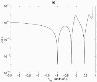
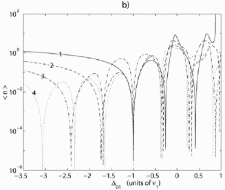
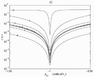
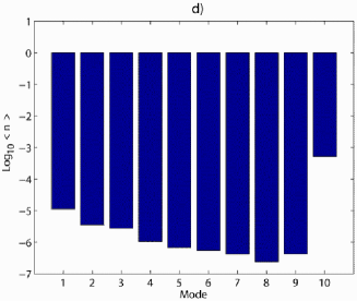
Figure 4: Raman sideband cooling a chain of 10 ions in the presence of a spatially inhomogeneous magnetic field such that the condition $\omega_{1}-\nu_{1}=\ldots=\omega_{N}-\nu_{N}$ is fulfilled (see Fig. 1). The parameters are $\Omega_{12}=100\times 2\pi$kHz, $\Omega_{01}=5\times 2\pi$kHz, $\Delta_{12}=-10\times 2\pi$MHz. The steady state mean vibrational excitation $\langle n^{(\alpha)}\rangle$ is displayed. a) $\langle n^{(1)}\rangle$ (COM mode) as a function of $\Delta_{01}$ in units of $\nu_{1}$. b) $\langle n^{(\alpha)}\rangle$ with $\alpha=1,2,3,4$ as function of $\Delta_{01}$. c) $\langle n^{(\alpha)}\rangle$ for $\alpha=1,\ldots,10$ as a function of $\Delta_{01}$. d) $\langle n^{(\alpha)}\rangle$ for $\alpha=1,\ldots,10$ when the chain is simultaneously cooled at the detuning $\Delta_{01}=-\nu_{1}$.

Figure 4b) displays $\langle n^{(1)}\rangle$, $\langle n^{(2)}\rangle$, $\langle n^{(3)}\rangle$, and $\langle n^{(4)}\rangle$ as a function of $\Delta_{01}$. These mean excitations have been calculated using the same parameters as in Fig. 4a). The minima visible in this figure can be identified with the corresponding resonances in the spectra of the ions by comparison with Fig. 1. A common minimum occurs at $\Delta_{01}=-\nu_{1}$ where all four vibrational modes are simultaneously cooled to low excitation numbers.

The mean vibrational quantum number $\langle n^{(\alpha)}\rangle$ of all ten axial modes is displayed in Fig. 4c) as a function of the detuning $\Delta_{01}$ in the neighborhood of the value $\Delta_{01}=-\nu_{1}$. At this value of $\Delta_{01}$ the mean excitation $\langle n^{(\alpha)}\rangle$ reaches its minimum for all modes. The mode at frequency $\nu_{10}$ displays a relatively narrow minimum and its mean vibrational number, although very small at exact resonance, is orders of magnitude larger than the ones of the other modes. In fact, ion 10 participates only little in the vibrational motion of mode 10. This is described by the small matrix element $S_{10}^{10}=0.0018$ that scales the corresponding Lamb-Dicke parameter as shown in Eq. (4).

Fig. 4d) displays the steady state temperature of each mode when the detuning of the Raman beams is set close to $-\nu_{1}$. At this detuning the average excitation reaches its minimum for each mode, which is $\langle n^{(\alpha)}\rangle<10^{-3}$.

III.2.1 Cooling rates for simultaneous Raman cooling

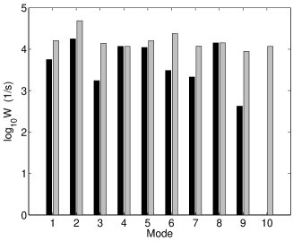
Figure 5: Cooling rates for Raman sideband cooling a chain of 10 ions in the presence of a spatially inhomogeneous magnetic field such that the condition $\omega_{1}-\nu_{1}=\ldots=\omega_{N}-\nu_{N}$ is fulfilled. The same parameters have been used here as for generating Fig. 3 ($\Omega_{12}=100\times 2\pi$kHz, $\Omega_{01}=30\times 2\pi$kHz, $\Delta_{12}=-10\times 2\pi$MHz). The black bars indicate the rate for each mode when simultaneously sideband cooling all modes. The grey bars give the cooling rates that are achieved, if (still in the presence of the magnetic field) the Raman detuning is set to that value where the maximum cooling rate for each individual mode is obtained.

We now turn to the cooling rates that are achieved when simultaneously cooling all modes, that is, the field gradient leading to the spectrum in Fig.1 is applied, and $\Delta_{01}=-\nu_{1}$. These rates are indicated by black bars in Fig. 5, and have been evaluated with the same parameters used for the simulation of sequential cooling in Fig. 3, that is, $\Omega_{01}=30\times 2\pi$kHz, $\Omega_{12}=100\times 2\pi$kHz, and $\Delta_{12}=-10\times 2\pi$MHz.

Figure 5 shows that the COM mode characterized by $\nu_{1}$ and the mode characterized by $\nu_{2}$ are cooled most efficiently, while modes 9 and 10 display much smaller cooling rates. In particular, $\Gamma_{\rm cool}^{(10)}\approx 10^{-1}$s^-1 which will make cooling of this mode very slow at $\Delta_{01}=-\nu_{1}$ .

The origin of this behaviour can be understood as follows. The scheme of simultaneous sideband cooling requires that each ion of the chain is employed to cool one of the axial modes. This is achieved by applying a suitable magnetic field gradient. The simplest experimental implementation uses a monotonically increasing magnetic field, such that the first ion of the chain is used for cooling mode 1, the second ion mode 2, etc. (compare Fig. 1). However, the coupling of a certain ion displacement to a certain mode can be very small. It occurs, for instance, that the largest axial excitations couple weakly to the ions at the edges of the ion string, instead they are mainly characterized by oscillations of ions in the center of the chain PRL04 . A manifestation of this behavior is the small value of the matrix element $S_{10}^{10}$. Thus, mode 10 is not efficiently cooled by illuminating ion 10, rather it is optimally cooled by addressing an ion closer to the center of the chain. This is evident by inspection of the grey bars in Fig. 5 that indicate the optimal cooling rate for each individual mode, obtained by employing that particular ion in the chain which has the largest coupling to the mode to be cooled. In presence of the magnetic field gradient, this optimal cooling rate is achieved, if the detuning, $\Delta_{01}$ is set such that the appropriate red-sideband transition of this particular ion is driven resonantly. In this way, the cooling rate is maximal for that particular mode (i.e., each grey bar corresponds to a different detuning).

For the case of mode 10 the difference between the cooling rates depending on which ion is addressed is particularly striking: the cooling rate of mode 10 at detuning $\Delta_{01}=-\nu_{1}$ (black bar) is very small, as noted above, whereas the optimal rate $\Gamma_{\rm cool}^{(10)}=2.63\times 10^{3}$s^-1 (given the parameters used here) is achieved at $\Delta_{01}=-3.28\times\nu_{1}$. At this detuning ion 6 is used for cooling mode 10, as can be seen from Fig. 1.

Efficient cooling of all modes, given the field gradient that gives rise to the spectrum illustrated in Fig. 1, can be obtained by combining sequential and simultaneous cooling as follows: First the ion string is illuminated with radiation such that $\Delta_{01}=-3.28\times\nu_{1}$ which will efficiently cool mode 10 and will have little effect on all other modes. Then, we apply radiation with $\Delta_{01}=-\nu_{1}$ (cooling rates indicated by black bars in Fig.  5). This will simultaneously cool all other modes. This is a specific recipe to cool 10 ions. For an arbitrary number of ions, first one cools the modes which cannot be efficiently simultaneously cooled with all other modes, and then, in a second step, as many modes as possible are cooled simultaneously (in our case modes 1 through 9).

A necessary condition for the efficiency of this scheme is

$$\Gamma_{\rm heat}^{(\alpha)}\ll\Gamma_{\rm cool,sim}^{(\alpha)}\ \forall\ \alpha=1,\ldots,10\ .$$ (15)

where $\Gamma_{\rm cool,sim}^{(\alpha)}$ is the cooling rate of mode $\alpha$ when simultaneously cooling it with the other modes. Condition (15) is the analogue to (9) which we derived for sequential cooling. Moreover, since in the scheme proposed here modes 1 through 9 are simultaneously cooled, a condition analogous to the one in Eq. (12) has to be fulfilled for mode 10 only: After mode 10 has been cooled, this mode may not heat up again appreciably during the time for which modes 1 through 9 are simultaneously cooled. This condition is expressed as

$$\Gamma_{\rm heat}^{(10)}\times T_{\rm sim}^{(10)}\ll 1\ .$$ (16)

where $T_{\rm sim}^{(10)}$ is the time during which modes 1 through 9 are cooled simultaneously to the desired final values, that is, the time during which mode 10 is not cooled and could heat up. Here, it is given by

$$T_{\rm sim}^{(10)}={\rm max_{\beta=1\ldots 9}}\left[\ln\frac{\langle n^{(\beta)}\rangle_{i}}{\langle n^{(\beta)}\rangle_{f}}/(\Gamma_{\rm cool}^{(\beta)}-\Gamma_{\rm heat}^{(\beta)})\right]\ ,$$ (17)

This relation is analogous to relation (11) for sequential cooling.

The times $T_{\rm seq}^{(10)}$ (eq. (11)) and $T_{\rm sim}^{(10)}$ (eq. (17)) give an upper limit for the tolerable trap heating rate of mode 10 for the cases of sequential and simultaneous cooling, respectively. It turns out that the relevant time scales $T_{\rm seq}^{(10)}$ and $T_{\rm sim}^{(10)}$ are of the same order of magnitude: Using eq. 17 to compute $T_{\rm sim}^{(10)}$ for the parameters used in Fig. 5 gives $T_{\rm sim}^{(10)}\approx\ln(\langle n\rangle_{i}/\langle n\rangle_{f})\times 2.4\times 10^{-3}$s, while $T_{\rm seq}^{(10)}\approx\ln(\langle n\rangle_{i}/\langle n\rangle_{f})\times 1.3\times 10^{-3}$s is obtained from eq. (11) for the same set of parameters footnoteC . Thus, the cooling scheme proposed here does not increase the admissible trap heating rate of mode 10. Since this rate is expected to be low anyway, this will not be a restriction prohibiting the successful cooling of a long ion chain using either sequential or simultaneous cooling.

III.3 Comparison of sequential and simultaneous cooling

So far we have stated the general conditions that have to be met in order to efficiently cool an ion chain with sequential cooling and with a scheme combining simultaneous and sequential sideband cooling. In this section we discuss their efficiencies.

We note that when using sequential sideband cooling, one may utilize all ions in the chain in order to cool one mode, where the cooling rates of each ion add up incoherently. In the case of simultaneous sideband cooling, on the other hand, only one ion is employed in order to cool a particular mode. Assuming that the coupling of this ion to the mode is sufficiently large to allow for efficient cooling, the following expression for the average simultaneous cooling rate is deduced

$$\Gamma_{\rm cool,sim}\approx\frac{1}{N}\Gamma_{\rm cool,seq}\$$ (18)

where $\Gamma_{\rm cool,seq}$ is the cooling rate for sequential cooling averaged over all modes. Thus, for simultaneous cooling relation (15) yields

$$\Gamma_{\rm heat}^{(\alpha)}\ll\frac{1}{N}\Gamma_{\rm cool,seq}\equiv\Gamma_{\rm<,sim}\ ,$$ (19)

From (18), since the total cooling rate is $\Gamma_{\rm<,seq}=\Gamma_{\rm cool,seq}/N$, one obtains that the efficiencies of simultaneous and sequential cooling are comparable. However, it should be remarked that this estimate corresponds to the worst case for simultaneous cooling. In fact, estimate (18) is correct for long-wavelength vibrational excitations, which correspond to low-frequency axial modes, where practically all ions of the chain participate in the mode oscillation. Short-wavelength excitations, on the other hand, are characterized by large displacements of the central ions, while the ions at the edges practically do not move PRL04 . Due to this property, for these modes one may find a magnetic field configuration such that $\Gamma_{\rm cool,sim}^{(\alpha)}\sim\Gamma_{\rm cool,seq}^{(\alpha)}$.

On the basis of these qualitative considerations, one may in general state that simultaneous cooling of the chain is at least as efficient as sequential cooling. For the configuration discussed in this paper the two methods are comparable. Differently from sequential cooling, however, the efficiency of simultaneous cooling can be substantially improved by choosing a suitable magnetic field configuration that maximizes coupling of each mode to one ion of the chain.

IV Sideband cooling using microwave fields

IV.1 Effective Lamb-Dicke parameter

We investigate now sideband cooling of the ion chain’s collective motion using microwave radiation for driving the sideband transition. It should be remarked that in this frequency range sideband excitation cannot be achieved by means of photon recoil which for long wavelengths is negligible. This is evident from eq. 4 using a typical trap frequency, $\nu_{\alpha}$ of the order $2\pi\times 1$MHz. Nevertheless, in Mintert01 it was shown that with the application of a magnetic field gradient an additional mechanical effect can be produced accompanying the absorption/emission of a photon. This is achieved by realizing different mechanical potentials for the states $|1\rangle$ and $|0\rangle$ Mintert01 ; Wunderlich02 ; Wunderlich03 . Hence, by changing an ion’s internal state by stimulated absorption or emission of a microwave photon the ion experiences a mechanical force.

An effective LDP can be associated with this force, that is defined as Wunderlich02 :

$$\eta_{j\alpha}^{\rm eff}\ e^{i\varphi_{j}}\equiv\eta_{j}^{\alpha}+i\varepsilon_{j}^{\alpha}$$ (20)

where

$$\varepsilon_{j}^{\alpha}=S_{j}^{\alpha}\frac{\partial_{z}\omega_{j}\,\Delta\!z_{\alpha}}{\nu_{\alpha}}\ ,$$ (21)

Here $\partial_{z}\omega_{j}$ is the spatial derivative of the resonance frequency of the ion at $z_{j}^{(0)}$ with respect to $z_{j}$, and $\Delta\!z_{\alpha}=\sqrt{\hbar/(2m\nu_{\alpha})}$. The reader is referred to the appendix for the theoretical description of the ion chain dynamics in presence of a spatially-varying magnetic field.

The term $\eta_{j}^{\alpha}$ appearing in Eq. (20) is the LDP due to photon recoil and defined in Eq. (4), while the term $\varepsilon_{j}^{\alpha}$ is the LPD arising from the mechanical effect induced by the magnetic field gradient. Their ratio is given by

$$\frac{\varepsilon_{j}^{\alpha}}{\eta_{j}^{\alpha}}=\frac{\kappa_{j}^{\alpha}}{k\Delta\!z_{\alpha}}=\frac{1}{2\pi}\frac{\lambda}{\Delta\!z_{\alpha}}\kappa_{j}^{\alpha}$$ (22)

where $\lambda$ is the wavelength of the considered transition and $\kappa_{j}^{\alpha}=\Delta\!z_{\alpha}\partial_{z}\omega_{j}/\nu_{\alpha}$ is the rescaled frequency gradient Mintert01 ; Wunderlich02 .

For a transition in the microwave frequency range, like the transition between the states $|0\rangle$ and $|1\rangle$ in ¹⁷¹Yb⁺, using typical values, like $\kappa_{j}^{\alpha}\approx 10^{-3}$, $\lambda\approx 10^{-2}$m, $\Delta\!z_{\alpha}\approx 10^{-8}$m, one finds that the Lamb-Dicke parameter due to the recoil of a microwave photon is at least two orders of magnitude smaller than the one due to the mechanical effect induced by the magnetic field, and thus $\eta_{j\alpha}^{\rm eff}\approx\varepsilon_{j}^{\alpha}$ in the microwave region.

IV.2 Steady state population and cooling rates

We study sideband cooling using microwave radiation using the model outlined in the appendix. For the Rabi frequencies the same parameters as in section III.2 are employed (i.e., $\Omega_{01}=5\times 2\pi$kHz, $\Omega_{12}=100\times 2\pi$kHz, $\Delta_{12}=-10\times 2\pi$MHz). The effective LDP is determined by the magnitude of the magnetic field gradient that is used to superimpose the motional sidebands of all vibrational modes, and is given by $\eta_{j\alpha}^{\rm eff}\approx\varepsilon_{j}^{\alpha}=S_{j}^{\alpha}\kappa_{j}^{\alpha}\approx S_{j}^{\alpha}\times 2\times 10^{-3}$.

It must be remarked that these parameters are outside the range of validity for the application of the numerical method we use. In fact, by applying it one neglects the fourth and sixth orders in the LDP expansion of the optical transition of the repumping cycle, which are of the same order of magnitude as the microwave sideband excitation. Nevertheless, given the complexity of the problem, characterized by a large number of degrees of freedom, we have chosen to use this simpler method in order to get an indicative estimate of the efficiency as compared to the case in which the sidebands are driven by optical radiation. Therefore, the results we obtain in this section are indicative. In fact, neglecting higher orders in the LDP of the optical transition corresponds to underestimate heating effects due to diffusion.

Fig. 6a) shows the steady state mean vibrational quantum number $\langle n^{(\alpha)}\rangle_{f}$ of the 10 axial vibrational modes as a function of the detuning $\Delta_{01}$ of the microwave radiation, where $\Delta_{01}=0$ when the microwave field is at frequency $\omega_{1}$. Figure 6b) displays the final excitation number of all vibrational modes as a function of $\Delta_{01}$ around the value $\Delta_{01}=-\nu_{1}$. Figure 6c) shows the steady state mean excitation of all 10 modes at $\Delta_{\mathrm{M}W}=-\nu_{1}$.

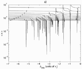
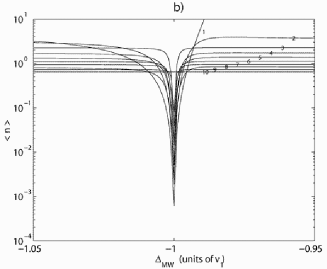
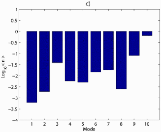
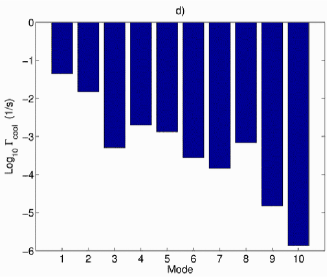
Figure 6: Microwave sideband cooling a chain of 10 ions in the presence of a spatially inhomogeneous magnetic field such that the condition $\omega_{1}-\nu_{1}=\ldots=\omega_{N}-\nu_{N}$ is fulfilled, that is, simultaneous sideband cooling using microwave radiation for sideband excitation. Same parameters as for Fig. 4 ($\Omega_{12}=100\times 2\pi$kHz, $\Omega_{01}=5\times 2\pi$kHz, $\Delta_{12}=-10\times 2\pi$MHz). a) Mean vibrational numbers $\langle n^{(\alpha)}\rangle_{f}$ at steady state as a function of the detuning $\Delta_{01}$. b) Same as a) for the values around $\Delta_{01}=-\nu_{1}$. c) $\langle n^{(\alpha)}\rangle_{f}$ at $\Delta_{01}=-\nu_{1}$, i.e. when all ten vibrational modes are simultaneously cooled. d) Cooling rates for $\Delta_{01}=-\nu_{1}$.

All vibrational modes are cooled close to their ground state. However, the average occupation number of the highest vibrational frequency $\nu_{10}$ is orders of magnitude larger than the ones of the other modes. The origin of this behavior is the small value of the coefficient $S_{10}^{10}=0.0018$ as is discussed in Sec. III.2. A comparison of Fig. 6c) with the results obtained by simultaneously cooling using an optical Raman processes (Fig. 4d) shows that the mean vibrational numbers that are achieved here are considerably larger.

In Fig. 6d) the cooling rates are displayed that are obtained when driving the sideband transition with microwave radiation. These rates are much smaller than the ones shown in Fig. 5 that are obtained using an optical Raman process.

From this comparison it is evident that simultaneous cooling is more effective by using an optical Raman process than microwave radiation. In particular, the cooling rates obtained with simultaneous microwave sideband cooling can be comparable to the heating rates in some experimental situations, resulting in inefficient cooling.

This striking difference in the efficiency can already be found, if comparing the two methods when they are applied to cooling a single ion. Its origin lies in the fact that in the optical case the LDP accounting for the photon recoil, namely $\eta_{j}^{\alpha}$ in Eq. (20), is considerably larger than the LDP, $\varepsilon_{j}^{\alpha}$ caused by the magnetic field gradient used here to superimpose the motional sidebands. This can be verified by using an optical wavelength in Eq. (22) which gives $\eta_{j\alpha}^{\rm eff}\approx\eta_{j}^{\alpha}$. On the other hand, driving the $|0\rangle-|1\rangle$ transition directly by microwaves results in $\eta_{j\alpha}^{\rm eff}\approx\varepsilon_{j}^{\alpha}\ll\eta_{j}^{\alpha}$. For the model system considered here, the optical LDP is at least one order of magnitude larger than the microwave LDP for simultaneous cooling.

In the microwave sideband cooling scheme optical transitions are used for repumping, thus leading to an enhanced diffusion rate during the dynamics and thus to lower efficiencies. The fundamental features of these dynamics can be illustrated by a rate equation of the form Eq. (5), describing sideband cooling of a single ion with microwave radiation, where the rates are

$$A_{-}=\frac{\Omega^{2}}{2\gamma}\Bigl{[}|\varepsilon|^{2}+\phi|\eta_{\rm opt}|^{2}\frac{\gamma^{2}}{4\nu^{2}+\gamma^{2}}\Bigr{]}$$ (23)

$$A_{+}=\frac{\Omega^{2}}{2\gamma}\Bigl{[}|\varepsilon|^{2}\frac{\gamma^{2}}{16\nu^{2}+\gamma^{2}}+\phi|\eta_{\rm opt}|^{2}\frac{\gamma^{2}}{4\nu^{2}+\gamma^{2}}\Bigr{]}\ ,$$ (24)

$\eta_{\rm opt}$ accounts for the recoil due to the spontaneous emission when the ion is optically pumped to the state $|0\rangle$ Morigi01 , and $\varepsilon$ is the LDP for the microwave transition due to the field gradient. The latter multiplies the terms where a sideband transition occurs by microwave excitation, whereas $\eta_{\rm opt}$ multiplies the terms where sideband excitation occurs by means of spontaneous emission, which thus describe the diffusion during the cooling process. Efficient ground state cooling is achieved when the rate of cooling is much larger than the rate of heating, which corresponds to the condition $A_{-}/A_{+}\gg 1$. For $\nu_{1}\gg\gamma_{\mu}$, whereby $\gamma_{\mu}$ is the linewidth of the $|0\rangle\to|1\rangle$ transition, this ratio scales as

$$\frac{A_{-}}{A_{+}}\sim\frac{|\varepsilon|^{2}}{|\eta_{\rm opt}|^{2}}\frac{4\nu^{2}}{\gamma^{2}}$$ (25)

This result differs for the ratio obtained in the all-optical case, where $A_{-}/A_{+}\sim 4\nu^{2}/\gamma^{2}$. For typical parameters, corresponding to a magnetic field gradient that superposes all sidebands in an ion trap, $|\varepsilon|\ll|\eta_{\rm opt}|$. Hence, for a given value of the ratio $\gamma/\nu$ the cooling efficiency in the optical case is considerably larger than in the microwave case.

Note that the parameter $\varepsilon$ can be made larger by increasing the magnitude of the magnetic field gradient, which in Eq. (22) corresponds to increasing $\kappa_{j}^{\alpha}$. However, if the modes of an ion chain are to be cooled simultaneously, the choice of the magnetic field gradient is fixed by the distance between neighboring ions, and the efficiency is thus limited by this requirement.

If an individual ion (or a neutral atom confined, for example, in an optical dipole trap) is to be sideband cooled, or sequential cooling is applied to a chain of ions, then the above mentioned restriction on the magnitude of $\varepsilon$ is not present and microwave sideband cooling can be as efficient as Raman cooling. For this case, method Marzoli94 may be implemented, provided the Lamb-Dicke regime applies and $\eta_{\rm opt}$ and $\epsilon$ are of the same order of magnitude.

V Experimental considerations

In this section we discuss how the magnetic field gradient for simultaneous sideband cooling can be generated and how cooling is affected, if the red motional sidebands of different vibrational modes are not perfectly superposed. In order to demonstrate the feasibility of the proposed scheme it is sufficient to restrict the discussion to very simple arrangements of magnetic field generating coils.

The use of a position dependent ac-Stark shift has been proposed in Staanum02 to modify the spectrum of a linear ion chain. This may be another way of appropriately shifting the sideband resonances but will not be considered here.

V.1 Required magnetic field gradient

If the vibrational resonances and the ions were equally spaced in frequency and position space, respectively, then a constant field gradient, appropriately chosen, could make all $N$ modes overlap and let them be cooled at the same time. Since $\nu_{\alpha}-\nu_{\alpha-1}$ decreases monotonically with growing $\alpha$ and the ions’ mutual distances vary with $z_{j}$, the magnetic field gradient has to be adjusted along the $z-$axis. The field gradient needed to shift the ions’ resonances by the desired amount is obtained from

$$\left.\frac{\partial B}{\partial z}\right|_{(z_{j}+z_{j-1})/2} \approx \frac{B(z_{j})-B(z_{j-1})}{z_{j}-z_{j-1}}$$ (26)

$$\stackrel{{\scriptstyle!}}{{=}} \frac{\upsilon_{j}-\upsilon_{j-1}}{\zeta_{j}-\zeta_{j-1}}\zeta_{0}\nu_{1}\frac{\hbar}{\mu_{B}},\ j=2,\ldots,N$$

where $\zeta_{j}\equiv z_{j}/\zeta_{0}$ is the scaled equilibrium position of ion $j$, and $\upsilon_{j}$ is the square root of the $j-$th eigenvalue of the dynamical matrix. Eq. 26 describes the situation for moderate magnetic fields (the Zeeman energy is much smaller than the hyperfine splitting), such that $\partial_{z}\omega_{j}=1/2\;g_{J}\mu_{B}\partial_{z}B$ with $g_{J}\approx g_{s}=2$ (state $|0\rangle$ does not depend on $B$). As an example, we consider again a string of $N=10$ ¹⁷¹Yb⁺ions in a trap characterized by $\nu_{z}=1\times 2\pi$MHz (thus, $\zeta_{0}=2.7\mu$m).

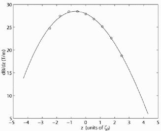
Figure 7: Required magnetic field gradient to superpose the motional red sidebands of ten ¹⁷¹Yb⁺ ions (markers) in a trap characterized by a COM frequency $\nu_{1}=1\times 2\pi$MHz and calculated field gradient (solid line) produced by three single wire windings (see text).

The markers in Fig. 7 indicate the values of the required field gradient according to eq. 26 whereas the solid line shows the gradient generated by 3 single windings of diameter 100$\mu$m, located at $z=-100,50,$ and $100$ mm $\approx 36\zeta_{0}$, respectively (the trap center is chosen as the origin of the coordinate system) Fortagh98 . Running the currents -5.33A, -6.46A, and 4.29A,respectively, through these coils produces the desired field gradient at the location of the ions. Micro electromagnets with dimensions of a few tens of micrometers and smaller are now routinely used in experiments where neutral atoms are trapped and manipulated Drndic98 . Current densities up to $10^{8}$A/cm² have been achieved in such experiments. A current density more than two orders of magnitude less than was achieved in atom trapping experiments would suffice in the above mentioned example.

This configuration of magnetic field coils shall serve as an example to illustrate the feasibility of the proposed cooling scheme in what follows. It will be shown that with such few current carrying elements in this simple arrangement one may obtain good results when simultaneously sideband cooling all axial modes. More sophisticated structures for generating the magnetic field gradients can of course be employed, making use of more coils, different diameters, variable currents, or completely different configurations of current carrying structures.

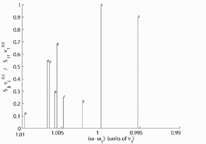
Figure 8: The vertical bars indicate the frequencies $\omega_{j}-\nu_{j}$ of first order sideband resonances corresponding to 10 axial vibrational modes of 10 ¹⁷¹Yb⁺ ions in an ion trap with the field gradient shown in Fig. 7. The frequencies are given relative to the transition frequency $\omega_{1}$ of the first ion, and the bars are labelled with $j=1,\ldots,10$. The height of the bars indicates the transition probability associated with a given sideband relative to the first sideband (COM mode) of ion 1 for a Raman transition. The relative transition probability is proportional to $|\eta_{j\alpha}^{\rm eff}|/|\eta_{11}^{\rm eff}|\approx S_{j}^{\alpha}\nu_{\alpha}^{-(1/2)}/S_{1}^{1}\nu_{1}^{-(1/2)}$ with $j=\alpha$

Ideally, all 10 sideband resonances would be superimposed for optimal cooling. The resonances shown in Fig. 8 result from the field gradient calculated using the simple field generating configuration described above, and do not all fall on top of each other. Nevertheless, Fig. 8 shows how well all 10 sideband resonances are grouped around $\omega_{1}-\nu_{1}$. Vertical bars indicate the location relative to $\omega_{1}$ of the red sideband resonance, $\omega_{j}-\nu_{j}$ of the $j-$th ion, with $j=1,\ldots,10$. These resonances all lie within a frequency interval of about $0.015\times\nu_{1}/2\pi=15$kHz.

The height of the bars in Fig. 8 indicates the strength of the coupling between the driving radiation and the respective sideband transition relative to the COM sideband of ion number 1. The relevant coupling parameter is the LDP. For optical transitions $|\eta_{j\alpha}^{\rm eff}|/|\eta_{11}^{\rm eff}|\approx|\eta_{j}^{\alpha}|/|\eta_{1}^{1}|=S_{j}^{\alpha}\nu_{\alpha}^{-(1/2)}/S_{1}^{1}\nu_{1}^{-(1/2)}$ with $j=\alpha$. The ratio of these parameters for the highest vibrational mode ($\alpha=10$) is about 3 orders of magnitude smaller than for mode 1, since ion 10 is only slightly displaced from its equilibrium position when mode 10 is excited (compare the discussion in section III.2).

We will now investigate how well simultaneous cooling can be done with the sideband resonances not perfectly superposed.

V.2 Simultaneous Raman cooling with non-ideal gradient

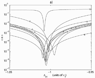
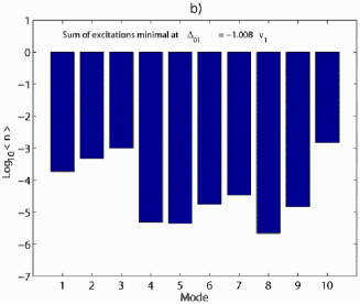
Figure 9: Raman sideband cooling a chain of 10 ions in the presence of a spatially inhomogeneous magnetic field. The condition $\omega_{1}-\nu_{1}=\ldots=\omega_{N}-\nu_{N}$ is approximately fulfilled (see Fig. 8). Same parameters as in Fig. 4 (i.e., $\Omega_{12}=100\times 2\pi$kHz, $\Omega_{01}=5\times 2\pi$kHz, $\Delta_{12}=-10\times 2\pi$MHz). a) Steady state vibrational excitation $\langle n^{(\alpha)}\rangle_{f}$ as a function of the detuning $\Delta_{01}$ around $\Delta_{01}=-\nu_{1}$. b) $\langle n^{(\alpha)}\rangle_{f}$ for each mode at that detuning where the sum of the mean vibrational quantum numbers of all ten modes is minimal.

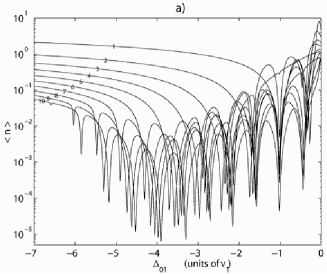
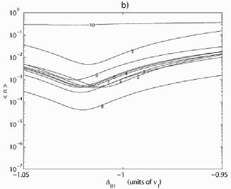
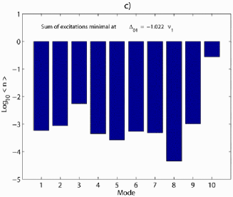
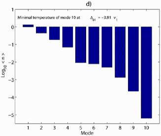
Figure 10: Raman sideband cooling a chain of 10 ions in the presence of a spatially inhomogeneous magnetic field. The condition $\omega_{1}-\nu_{1}=\ldots=\omega_{N}-\nu_{N}$ is approximately fulfilled (see Fig. 8). a) $\langle n^{(\alpha)}\rangle_{f}$ as a function of $\Delta_{01}$ displaying all first order red sidebands with all parameters unchanged compared to Fig. 9 except $\Omega_{12}=1\times 2\pi$MHz. b) $\langle n^{(\alpha)}\rangle_{f}$ as a function of $\Delta_{01}$ in the vicinity of the common sideband resonance around $\Delta_{01}=-\nu_{1}$. The resonances are power broadened and ac-Stark shifted compared to the ones in Fig. 9a). c) Steady state population $\langle n^{(\alpha)}\rangle_{f}$ for each mode at that detuning where the sum of the mean vibrational quantum numbers of all ten modes is minimal (the analogue to Fig. 9b except that $\Omega_{12}=1\times 2\pi$MHz.) d) $\langle n^{(\alpha)}\rangle_{f}$ for each mode at that detuning where one of the modes (here mode 10) reaches the absolute minimum. Optimal cooling of all vibrational modes is achieved by first cooling mode 10 at $\Delta_{01}=-3.91\nu_{1}$ and subsequently modes 1 through 9 at $\Delta_{01}=-1.022\nu_{1}$.

In Fig. 9a) the steady state vibrational excitation, $\langle n^{(\alpha)}\rangle_{f}$ of a string of 10 ions is displayed as a function of the detuning of the Raman beams relative to the resonance frequency $\omega_{1}$ of ion 1. The Rabi frequencies and detuning, too, are the same as have been used to generate Fig. 4. However, the field gradient that shifts the ions’ resonances is not assumed ideal as in Fig. 4, instead the one generated by three single windings as described above (Fig. 7) has been used. Despite the imperfect superposition of the cooling resonances, low temperatures of all modes close to their ground state can be achieved as can be seen in Fig. 9b). Here, the value of $\langle n^{(\alpha)}\rangle_{f}$ for each mode has been plotted at that detuning $\Delta_{01}=-1.008\nu_{1}$ where the sum of all excitations is minimal.

Fig. 10a displays the excitation of each mode over a wide range of the detuning such that all first order red sideband resonances are visible. Here, the Rabi frequency $\Omega_{12}$ of the repump laser has been increased to $1\times 2\pi$MHz as compared to $100\times 2\pi$kHz in the previous figures. This results i) in higher final temperatures, and, ii) in broader resonances as is evident in Fig. 10b and thus makes cooling less susceptible to errors in the relative detuning between laser light and ionic resonances.

A higher steady state vibrational excitation due to the larger intensity of the repump laser is evident in Fig. 10c where $\langle n^{(\alpha)}\rangle_{f}$ for each mode is plotted with the same parameters as in Fig. 9b, however with $\Omega_{12}=1\times 2\pi$MHz.

Errors and fluctuations in the relative detuning of the Raman laser beams driving the sideband transition are expected to be small and not to affect the efficiency of simultaneous cooling, if the two light fields inducing the stimulated Raman process are derived from the same laser source using, for example, acousto-optic or electro-optic modulators. This is feasible by translating into the optical domain the microwave or radio frequency that characterizes the splitting of states $|0\rangle$ and $|1\rangle$. Microwave or rf signals can be controlled with high precision and display low enough drift to ensure efficient cooling. If a large enough intensity of the repump laser is employed, then the steady state vibrational excitation varies slowly as a function of $\Delta_{01}$ as is visible in Fig. 10b. Thus, the requirements regarding both the precision of adjustment and the drift of the source generating the Raman difference frequency are further relaxed.

It should be noted that efficient cooling does not only occur around the resonance $\Delta_{01}=-\nu_{1}$ but also at other values of $\Delta_{01}$ as can be seen in Fig. 10a. As an example, Fig. 10d shows $\langle n^{(\alpha)}\rangle_{f}$ of all modes at that detuning, $\Delta_{01}=-3.91\nu_{1}$ where mode 10 reaches its absolute minimum. At this resonance the red sideband of the 5th ion corresponding to the 10th mode is driven by the Raman beams (compare Fig. 1). Note that all other vibrational modes are also cooled at the same time. Therefore, an efficient procedure for cooling all vibrational modes close to their ground state would be to first tune the Raman beams such that mode 10 is optimally cooled (i.e., $\Delta_{01}=-3.91\nu_{1}$, Fig. 10d), and subsequently set $\Delta_{01}=-1.022\nu_{1}$ (Fig. 10c) in order to simultaneously cool modes 1 through 9. This approach is discussed in more detail in section III.2.1.

Initial cooling of vibrational modes often is prerequisite for subsequent coherent manipulation of internal and motional degrees of freedom of an ion chain, for example, quantum logic operations. When implementing quantum logic operations it may not be advantageous to address all motional sidebands with a single frequency as is done here for simultaneous sideband cooling. The magnetic field gradient that superposes the sideband resonances for cooling may then be turned off adiabatically after initial Raman cooling of all vibrational modes. This should be done fast enough not to allow for appreciable heating of the ion string, for example, by patch fields, and slow enough not to excite vibrational modes in the process. A lower limit for the time it takes to ramp up the gradient seems to be $2\pi/\nu_{1}$. Thus, with $\nu_{1}=1\times 2\pi$MHz the additional time needed to change the field gradient is negligible compared to the time needed to sideband cool the ion string which for typical parameters takes between a few hundred $\mu$s and a few ms (compare Fig. 5).

If microwave radiation is used to coherently manipulate internal and motional degrees of freedom and for quantum logic operations, it is useful not to turn off the magnetic field gradient, but instead to ramp up the field gradient to a value where all coincidences between internal and motional resonances are removed Mintert01 ; Wunderlich03 . Also, a larger field gradient for quantum logic operations is desirable in this case to have stronger coupling between internal and external states (i.e., a larger effective LDP $\eta_{j\alpha}^{\rm eff}$ [eq. 20]). The considerations in the previous paragraph regarding the time scale of change of the field gradient apply here, too.

For the cooling scheme introduced here to work, the field gradient has to vary in the axial direction and it remains to be shown in what follows that this variation is compatible with the neglect of higher-order terms in the local displacement $q_{j}$ of ion $j$ and in $\partial_{z}B$ in the derivation of the effective Lamb-Dicke parameter induced by the magnetic field gradient Mintert01 ; Wunderlich02 . Neglecting higher order terms is justified as long as $|q_{j}^{2}\partial_{z}^{2}B|\ll|q_{j}\partial_{z}B|$. Using 26 and $q_{j}\approx\Delta\!z=\sqrt{\hbar/2m\nu_{1}}$ this condition can be written as

$$\frac{2}{\zeta_{j+1}-\zeta_{j-1}}\left|\frac{(\upsilon_{j+1}-\upsilon_{j})(\zeta_{j}-\zeta_{j-1})}{(\upsilon_{j}-\upsilon_{j-1})(\zeta_{j+1}-\zeta_{j})}-1\right|\ll\frac{\zeta_{0}}{\Delta\!z}\;.$$ (27)

Considering the region where the second derivative of the magentic field is maximal ($j=9$) and inserting numbers into relation 27 gives for ten ions $0.24\ll 2.9\times 10^{3}(m/\nu_{1})^{\frac{1}{6}}$. The right-hand side of this inequality is dimensionless if $m$ is inserted in a.m.u., and yields $\approx 500$ for ¹⁷¹Yb⁺ions and $\nu_{1}=1\times 2\pi$MHz. Hence, relation 27 is fulfilled. This can be understood by considering that the typical distance, $\zeta_{0}$ over which the gradient has to vary is much larger than the range of motion, $q_{j}\approx\Delta\!z$ of an individual ion, and the approximation of a linear field gradient is a good one.

VI Conclusions

We have proposed a scheme for cooling the vibrational motion of ions in a linear trap configuration. Axial vibrational modes are simultaneously cooled close to their ground state by superimposing the red motional sidebands in the absorption spectrum of different ions such that the red sideband of each mode is excited when driving an internal transition of the ions with monochromatic radiation. This spectral property is achieved by applying a magnetic field gradient along the trap axis shifting individually the internal ionic resonances by a desired amount.

Exemplary results of numerical simulations for the case of an ion chain consisting of $N=10$ ions are presented and extensively discussed. Detailed simulations have also been carried out with $1<N<10$ and for some values $N>10$. They lead to the same qualitative conclusion as presented for the case of $N=10$.

Numerical studies show that simultaneously Raman cooling all axial modes is effective for realistic sets of parameters. These studies also reveal that using microwave radiation to drive the sideband transition is not as efficient, due to the relatively small mechanical effect associated with the excitation of this transition. The mechanical effect could be enhanced by applying a larger magnetic field gradients. For simultaneous sideband cooling of all vibrational modes, however, the gradient is fixed by the requirement of superimposing the sidebands. Usual sideband cooling on a hyperfine or Zeeman transition using microwave radiation becomes possible, if a larger field gradient is used. This may be particularly useful, if a single ion (or an atom in an optical dipole trap) is to be sideband cooled using a microwave transition, or, if the vibrational modes of an ion chain are to be cooled sequentially using microwave radiation. Moreover, these techniques could also be implemented for sympathetic cooling of an ion chain, whereby some modes are simultaneously cooled by addressing ions of other species embedded in the chain Morigi01 ; Kielpinski01 ; Barrett03 .

In conclusion, we have shown that simultaneous sideband cooling with optical radiation can be efficiently implemented taking into account experimental conditions and even for a simple arrangement of magnetic field generating elements.

VII Acknowledgements

We acknowledge financial support by the Deutsche Forschungsgemeinschaft, Science Foundation Ireland under Grant No. 03/IN3/I397, and the European Union (QGATES,QUIPROCONE).

VIII Appendix

In this appendix we introduce the hamiltonian and master equation describing the dynamics discussed in Sec. IV.2. We consider a chain consisting of $N$ identical ions aligned along the $z$-axis, and in presence of a magnetic field $B(z)$. The internal electronic states of each ion which are relevant for the dynamics are the stable states $|0\rangle$ and $|1\rangle$ and the excited state $|2\rangle$. The transitions $|0\rangle\to|1\rangle$, $|1\rangle\to|2\rangle$ are respectively a magnetic and an optical dipole transition. We assume that the magnetic moments of $|0\rangle$ and $|2\rangle$ vanish, while $|1\rangle$ has magnetic moment $\mu$. Thus its energy with respect to $|0\rangle$ is shifted proportionally to the field, $\hbar\omega_{0}(z)\propto|B(z)|$. The Hamiltonian describing the internal degrees of freedom has the form:

$$H_{\rm int}=\hbar\sum_{j}\left(\omega_{0}(z_{j})|1\rangle_{j}\langle 1|+\omega_{2}|2\rangle_{j}\langle 2|\right)$$ (28)

where the index $j$ labels the ions along the chain. The collective excitations of the chain are described by the eigenmodes at frequency $\nu_{1},\ldots,\nu_{N}$, which are independent of the internal states. Denoting with $Q_{\alpha},P_{\alpha}$ the normal coordinates and conjugate momenta of the oscillator at frequency $\nu_{\alpha}$, the Hamiltonian for the external degrees of freedom then has the form

$$H_{\rm mec} = \frac{1}{2m}\sum_{\alpha=1}^{N}P_{\alpha}^{2}$$

$$+\frac{m}{2}\sum_{\alpha=1}^{N}\nu_{\alpha}^{2}\left[Q_{\alpha}+\frac{\hbar}{2m\nu_{\alpha}^{2}}\sum_{j}\left.\frac{\partial\omega_{j}}{\partial z_{j}}\right|_{z_{0,j}}|1\rangle\langle 1|S_{j}^{\alpha}\right]^{2}$$

where we have neglected the higher spatial derivatives of the magnetic field.

Thus, the coupling of the excited state $|1\rangle$ to a spatially varying magnetic field shifts the center of the oscillators for the ions in the electronic excited state.
The states $|0\rangle$ and $|1\rangle$ are coupled by radiation according to the Hamiltonian

$$W_{01}=\sum_{j}\frac{\hbar\Omega_{01}}{2}\left[|1\rangle_{j}\langle 0|{\rm e}^{-{\rm i}(\omega_{01}t-k_{01}z_{j}+\psi)}+{\rm H.c.}\right]$$ (30)

where the coupling can be generated either by microwave radiation driving the magnetic dipole, or by a pair of Raman lasers. In the first case, $\Omega_{01}$ is the Rabi frequency, $\omega_{01}$ the frequency of radiation and $k_{01}$ the corresponding wave vector. In the case of coupling by Raman lasers, $\Omega_{01}$ is the effective Rabi frequency, $\omega_{01}$ the frequency and $k_{01}$ the resulting wave vector describing the two-photon process.
The transition $|1\rangle\to|2\rangle$ is driven below saturation by a laser at Rabi frequency $\Omega_{12}$, frequency $\omega_{12}$, and wave vector $k$. The interaction term reads:

$$W_{12}=\sum_{j}\frac{\hbar\Omega_{12}}{2}\left[|2\rangle_{j}\langle 1|{\rm e}^{-{\rm i}(\omega_{12}t-kz_{j}+\psi)}{\rm e}^{{\rm i}kq_{j}}+{\rm H.c.}\right]$$ (31)

where $q_{j}$ is the displacement of the ion $j$ from the classical equilibrium position $z_{j}$.
The master equation for the density matrix $\rho$, describing the internal and external degrees of freedom of the ions, reads:

$$\frac{\partial}{\partial t}\rho=\frac{1}{{\rm i}\hbar}[H,\rho]+{\cal L}\rho$$ (32)

where $H=H_{0}+H_{\rm mec}+W_{01}+W_{12}$, and ${\cal L}\rho$ is the Liouvillian describing the spontaneous emission processes, i.e. the decay from the state $|2\rangle$ into the states $|0\rangle$ and $|1\rangle$ at rates $\Gamma_{20}$, $\Gamma_{21}$, respectively, where $\Gamma=\Gamma_{20}+\Gamma_{21}$ is the total decay rate. The Liouville operator for the spontaneous decay is

$${\cal L}\rho=-\frac{1}{2}\Gamma\sum_{j}\Bigl{[}|2\rangle_{j}\langle 2|\rho+\rho|2\rangle_{j}\langle 2|\Bigr{]}$$ (33)

$$+\Gamma_{20}\int_{-1}^{1}{\rm d}u{\cal N}(u){\rm e}^{{\rm i}kuq_{j}}|0\rangle_{j}\langle 2|\rho|2\rangle_{j}\langle 0|{\rm e}^{-{\rm i}kuq_{j}}$$

$$+\Gamma_{21}\int_{-1}^{1}{\rm d}u{\cal N}(u){\rm e}^{{\rm i}kuq_{j}}|1\rangle_{j}\langle 2|\rho|2\rangle_{j}\langle 1|{\rm e}^{-{\rm i}kuq_{j}}$$

with ${\cal N}(u)$ the dipole pattern for spontaneous emission and $u$ the projection of the direction of photon emission onto the trap axis. In order to study the dynamics, it is convenient to move to the inertial frames rotating at the field frequencies. Moreover, we apply the unitary transformation Wunderlich02

$$U=\exp\left[-{\rm i}\sum_{\alpha}\left(\frac{1}{2m\nu_{\alpha}^{2}}\sum_{j}\left.\frac{\partial\omega_{0,j}}{\partial z_{j}}\right|_{z_{0,n}}|1\rangle_{j}\langle 1|S_{j}^{\alpha}\right)P_{\alpha}\right]$$ (34)

We denote with $\tilde{\rho}$ the density matrix in the new reference frame. The master equation now reads

$$\frac{\partial}{\partial t}\tilde{\rho}=\frac{1}{{\rm i}\hbar}[\tilde{H},\tilde{\rho}]+{\cal L}\tilde{\rho}$$ (35)

where $\tilde{H}=\tilde{H}_{0}+\tilde{H}_{\rm mec}+\tilde{W}_{01}+\tilde{W}_{12}$, and the individual terms have the form:

$$\tilde{H_{0}}=\hbar\sum_{j}\left[\delta(z_{j})|0\rangle_{j}\langle 0|+\Delta(z_{j})|2\rangle\langle 2|\right]$$ (36)

with $\delta(z_{j})=\omega_{01}-\omega_{0}(z_{j})$ and $\Delta(z_{j})=\omega_{2}-\omega_{0}(z_{j})-\omega_{12}$. The mechanical energy is

$$\tilde{H}_{\rm mec} = \frac{1}{2m}\sum_{\alpha=1}^{N}P_{\alpha}^{2}+\frac{m}{2}\sum_{\alpha=1}^{N}\nu_{\alpha}^{2}Q_{\alpha}^{2}$$ (37)

$$= \sum_{\alpha}\hbar\nu_{\alpha}\left(a^{\dagger}_{\alpha}a_{\alpha}+\frac{1}{2}\right)$$

where $a^{\dagger}_{\alpha}$, $a_{\alpha}$ are the creation and annihilation operator, respectively of a quantum of energy $\hbar\nu_{\alpha}$. The interaction term between the states $|0\rangle$ and $|1\rangle$ now reads

$$\tilde{W}_{01}=\sum_{j}\frac{\hbar\Omega_{01}}{2}\left[|1\rangle_{j}\langle 0|{\rm e}^{{\rm i}(k_{01}z_{j}-\psi)}\prod_{\alpha}{\rm e}^{-{\rm i}\tilde{k}_{j}^{\alpha}P_{\alpha}}+{\rm H.c}\right]$$ (38)

where

$$\tilde{k}_{j}^{\alpha}=\frac{\partial\omega_{0,j}}{\partial z_{j}}\frac{1}{2m\nu_{\alpha}^{2}}S_{j}^{\alpha}$$ (39)

Thus, the excitation between two states, where the mechanical potential in one is shifted with respect to the other, corresponds to an effective recoil, here described by the effective Lamb-Dicke parameter $\tilde{\eta}_{j}^{\alpha}=\tilde{k}_{j}^{\alpha}\sqrt{\hbar m\nu_{\alpha}/2}$. Finally, the optical pumping between the states $|1\rangle$ and $|2\rangle$ is given by

$$\tilde{W}_{12}=\sum_{j}\frac{\hbar\Omega_{12}}{2}\left[|2\rangle_{j}\langle 1|{\rm e}^{{\rm i}\chi_{j}}\prod_{\alpha}{\rm e}^{{\rm i}(\eta^{\rm eff}_{j\alpha}a^{\dagger}_{\alpha}+\eta^{{\rm eff}*}_{j\alpha}a_{\alpha})}+{\rm H.c.}\right]$$ (40)

where $\chi_{j}$ is a constant phase, that depends on the position according to

$$\chi_{j}=kz_{j}-\psi-\hbar k\sum_{\alpha}\tilde{k}_{j}^{\alpha}S_{j}^{\alpha}/2$$ (41)

and $\eta^{\rm eff}_{j\alpha}$ is an effective Lamb-Dicke parameter defined in Eq. (20). The dynamics of the individual modes are effectively decoupled from the others in the Lamb-Dicke regime, which holds when the condition $|\eta^{\rm eff}_{j\alpha}|\sqrt{\langle n^{\alpha}\rangle}\ll 1$ is fulfilled.

The cooling rate and steady state occupation are evaluated for each mode by using the procedure outlined in Marzoli94 . The rates $A_{\pm}^{\alpha}$, which determine the cooling rate and the steady state mean occupation according to Eqs. (7) and (8), are given by

$$A_{\pm}^{\alpha}=2{\rm Re}\{S_{\alpha}(\mp\nu_{\alpha})+D_{\alpha}\}$$ (42)

where $S_{\alpha}(\mp\nu_{\alpha})$ is the fluctuation spectrum of the dipole force $F_{j,\alpha}$,

$$S_{\alpha}(\pm\nu_{\alpha})=\frac{1}{M\nu_{\alpha}}\sum_{j}\int_{0}^{\infty}{\rm d}t{\rm e}^{\pm{\rm i}\nu_{\alpha}t}{\rm Tr}\{F_{j,\alpha}(t)F_{j,\alpha}(0)\rho_{\rm St}\}$$ (43)

and $D_{\alpha}$ is the diffusion coefficient due to spontaneous emission,

$$D_{\alpha}=\phi\sum_{j}\left(|{\eta_{20}}_{\alpha}^{j}|^{2}\Gamma_{20}+|{\eta_{12}}_{\alpha}^{j}|^{2}\Gamma_{21}\right)\langle 2|\rho_{\rm St}|2\rangle$$ (44)

where $\phi=\int du{\cal N}(u)u^{2}$ and here $\phi=2/5$. Here, $\rho_{\rm St}$ is the stationary solution of Eq. (35) at zero order in the Lamb-Dicke parameter, and the dipole force $F_{j,\alpha}$ is defined as

$$F_{j,\alpha}={\rm i}{\eta_{01}}_{\alpha}^{j}\frac{\Omega_{01}}{2}|1\rangle\langle 0|+{\rm i}{\eta_{12}}_{\alpha}^{j}\frac{\Omega_{12}}{2}|2\rangle\langle 1|+{\rm H.c.}$$ (45)

The fluctuation spectrum and the diffusion are found by evaluating numerically the steady state density matrix. The two-time correlation function in (43) is found by applying the quantum regression theorem according to the master equation (35) at zero order in the Lamb-Dicke parameter.

References

- (1) C. Myatt, B. King, Q. Turchettte, C. Sackett, D. Kielpinski, W. Itano, C. Monroe, and D. Wineland, Nature 403, 269 (2000).
- (2) C. Roos, T. Zeiger, H. Rohde, H. Nägerl, J. Eschner, D. Leibfried, F. Schmidt-Kaler, and R. Blatt, Phys. Rev. Lett. 83, 4713 (1999).
- (3) T. Hannemann, D. Reiß, C. Balzer, W. Neuhauser, P. E. Toschek, and C. Wunderlich, Phys. Rev. A 65, 050303(R) (2002).
- (4) Ch. Wunderlich and Ch. Balzer, Adv. At. Mol. Opt. Phys. 49, 293 (2003).
- (5) C. A. Sackett, D. Kielpinski, B. E. King, C. Langer, V. Meyer, C. J. Myatt, M. Rowe, Q. A. Turchette, W. M. Itano, D. J. Wineland, and C. Monroe, Nature 404, 256 (2000). C.F. Roos, M. Riebe, H. Häffner, W. Hänsel, J. Benhelm, G.P.T. Lancaster, C. Becher, F. Schmidt-Kaler, R. Blatt, Science 304, 1478 (2004).
- (6) J. I. Cirac and P. Zoller, Phys. Rev. Lett. 74, 4091 (1995).
- (7) F. Schmidt-Kaler, H. Häffner, M. Riebe, S. Gulde, G.P.T. Lancaster, T. Deuschle, C. Becher, C.F. Roos, J. Eschner, R. Blatt, Nature 422, 408 (2003); D. Leibfried, B. Demarco, V. Meyer, D. Lukas, M. Barrett, J. Britton, B. Jelenkovic, C. Langer, T. Rosenband, D.J. Wineland, Nature 422, 412 (2003).
- (8) M. Riebe, H. Häffner, C.F. Roos, W. Hänsel, J. Benhelm, G.P.T. Lancaster, T.W. Körber, C. Becher, F. Schmidt-Kaler, D.F.V. James, R. Blatt, Nature 429, 734 (2004); M.D. Barrett, J. Chiaverini, T. Schaetz, J. Britton, W.M. Itano, J.D. Jost, E. Knill, C. Langer, D. Leibfried, R. Ozeri, and D.J. Wineland, Nature 429, 737 (2004)
- (9) A. Sorensen and K. Molmer, Phys. Rev. A 62, 022311 (2000).
- (10) D. Jonathan, M. B. Plenio, and P. L. Knight, Phys. Rev. A 62, 042307 (2000).
- (11) D. J. Wineland, C. Monroe, W. M. Itano, D. Leibfried, B. E. King, and D. M. Meekhof, J. Res. Natl. Inst. Stand. Technol. 103, 259 (1998).
- (12) B. E. King, C. S. Wood, C. J. Myatt, Q. A. Turchette, D. Leibfried, W. M. Itano, C. Monroe, and D. J. Wineland, Phys. Rev. Lett. 81, 1525 (1998).
- (13) E. Peik, J. Abel, T. Becker, J. von Zanthier, and H. Walther, Phys. Rev. A 60, 439 (1999).
- (14) C. F. Roos, D. Leibfried, A. Mundt, F. Schmidt-Kaler, J. Eschner, and R. Blatt, Phys. Rev. Lett. 85, 5547 (2000).
- (15) D. Reiß, K. Abich, W. Neuhauser, C. Wunderlich, and P. E. Toschek, Phys. Rev. A 65, 053401 (2002).
- (16) J. Eschner, G. Morigi, F. Schmidt-Kaler, and R. Blatt, J. Opt. Soc. Am. B 20, 1003 (2003).
- (17) D. Kielpinski, C. Monroe, and D. J. Wineland, Nature 417, 709 (2002).
- (18) F. Mintert and C. Wunderlich, Phys. Rev. Lett. 87, 257904 (2001).
- (19) C. Wunderlich, in Laser Physics at the Limit (Springer Verlag, Heidelberg-Berlin-New York, 2001), pp. 261–271.
- (20) D. Mc Hugh and J. Twamley, Phys. Rev. A 71, 012315 (2005).
- (21) Strong radial confinement can be achieved in a linear Paul trap Ghosh95 by applying an rf voltage to the quadrupole electrodes while the weaker trapping potential along the axis is generated by a dc voltage. Another possible realization of a trap potential having the described symmetry can be obtained with a Penning trap Ghosh95 ; Powell02 .
- (22) P. K. Ghosh, Ion Traps (Clarendon Press, Oxford, 1995), Chap. 2.
- (23) H.F. Powell, D. M. Segal, and R. C. Thompson, Phys. Rev. Lett. 89, 093003 (2002).
- (24) A. Steane, Appl. Phys. B 64, 623 (1997).
- (25) D. F. V. James, Appl Phys. B 66, 181 (1998).
- (26) S. Stenholm, Rev. Mod. Phys. 58, 699 (1986).
- (27) G. Morigi and H. Walther, Eur. Phys. J. D 13, 261 (2001).
- (28) G. Morigi, J. Eschner, J. Cirac, and P. Zoller, Phys. Rev. A 59, 3797 (1999).
- (29) The selection rules actually prohibit a direct radiative transition between and , which in this case correspond to the 171Yb+states P and S, respectively. Here, we assume that a field is present, coupling P and P, thus allowing to have a transition from P to S with adjustable rate.
- (30) I. Marzoli, J. Cirac, R. Blatt, and P. Zoller, Phys. Rev. A 49, 2771 (1994).
- (31) D. Reiß, A. Lindner, and R. Blatt, Phys. Rev. A 54, 5133 (1996).
- (32) Q.A. Turchette et al., Phys. Rev. A 61, 063418 (2000).
- (33) G. Morigi, J. Eschner, C.H. Keitel, Phys. Rev. Lett. 85, 4458 (2000); G. Morigi, Phys. Rev. A 67, 033502 (2003).
- (34) G. Morigi and Sh. Fishman, Phys. Rev. Lett. 93, 170602 (2004).
- (35) Experimental data on the heating rates of each individual mode for 10 ions seem not to be available. For the purpose of computing the relevant time scales for simultaneous and sequential cooling therefore, the heating rates were set to zero in equations 11 and 17. For simplicity it was assumed that and take on the same value for each mode.
- (36) Peter Staanum and Michael Drewsen, Phys. Rev. A 66, 040302(R) (2002).
- (37) Wires with rather small diameter can be used for these coils when they are in contact with a suitable heat sink. See, for instance: J. Fortagh, A. Grossmann, C. Zimmermann, T. W. Hänsch: Phys. Rev. Lett. 81, 5310 (1998).
- (38) For example, M. Drndic, K. Johnson, J. H. Thywissen, M. Prentiss, and R. Westervelt, Appl. Phys. Lett. 72, 2906 (1998); J. Reichel, W. Hänsel, and T. W. Hänsch, Phys. Rev. Lett. 83, 3398 (1999).
- (39) D. Kielpinski, B.E. King, C.J. Myatt, C.A. Sackett, Q.A. Turchette, W.M. Itano, C. Monroe, D.J. Wineland, and W.H. Zurek, Phys. Rev. A 61, 032310 (2000).
- (40) M.D. Barrett, B. DeMarco, T. Schaetz, V. Meyer, D. Leibfried, J. Britton, J. Chiaverini, W.M. Itano, B. Jelenkovic, J.D. Jost, C. Langer, T. Rosenband, and D.J. Wineland Phys. Rev. A 68, 042302 (2003)