Sampling errors of correlograms with and without sample mean removal for higher-order complex white noise with arbitrary mean

Abstract

We derive the bias, variance, covariance, and mean square error of the standard lag windowed correlogram estimator both with and without sample mean removal for complex white noise with an arbitrary mean. We find that the arbitrary mean introduces lag dependent covariance between different lags of the correlogram estimates in spite of the lack of covariance in white noise for non-zeros lags. We provide a heuristic rule for when the sample mean should be, and when it should not be, removed if the true mean is not known. The sampling properties derived here are useful is assesing the general statistical performance of autocovariance and autocorrelation estimators in different parameter regimes. Alternatively, the sampling properties could be used as bounds on the detection of a weak signal in general white noise.

1 Introduction

The correlogram, an estimate of the autocorrelation function (ACF) of a time series, is one of the cornerstone analyses in the signal processing toolbox and therefore an understanding of its statistical errors for various random signals is of fundamental importance. Since the first published work [2] the sampling properties of various ACF estimators for a wide variety of different processes have been investigated [6, 5, 1]. Yet it seems that one fundamental process has not draw full attention: general independent and identically distributed (IID) processes. In particular, IID processes introduce two novel aspects to the statistical errors of ACF estimators: a non-zero mean and non-analytic signals.

In order to investigate these novel effects and in particular the non-zero mean in particular, we compare the standard correlogram estimator both with and without sample mean subtracted from the data samples. These two estimators are introduced in section 2.1 and section 2.2 respectively. We conclude by discussing how to treat the mean of a process when estimating correlation.

Our main finding is that an unknown mean introduces non-zero lag dependent covariance irrespective of whether the sample mean is removed or not. This is surprising seeing that white noise signals are not non-zero dependent.

2 Lag windowed correlogram estimators

In dealing with an uncertain mean when estimating the autocovariance of a give sequence of data there are two possible procedures: either one estimates the mean from the given data or the mean can be guessed in some way not based on the given data. These two procedures taken together with the subsequent correlogram computation can be seen as two different types of autocovariance estimators. That is, there are autocovariance estimators that include some sort of mean estimation and there correlograms that do not. In what follows we consider one version of each, namely, we consider the standard windowed correlogram and the standard windowed correlogram with sample mean removal.

2.1 Estimator without sample mean removal

The classical correlogram does not involve any explicit mean estimation. Allowing for lag windowing, we define it for positive lags as

$$\widehat{R}_{zz}^{(\mu)}[l]:=\mathcal{W}[l]\sum_{k=1}^{N-l}z^{*}[k]z[k+l],\quad l=0,1,2...N-1,$$ (1)

where $z[1],z[2],...z[N]$ are possibly complex data samples, $N$ is the number of data samples, $\mathcal{W}[l]$ is an arbitrary real valued lag weighting function, and $z^{*}$ denotes the complex conjugate of $z$. We use square brackets $[\cdot]$ to refer to a function of a discrete valued variable.

There are two standard choices for $\mathcal{W}[l]$. If

$$\mathcal{W}[l]=\mathcal{W}_{U}[l]:=\frac{1}{N-|l|}$$ (2)

the estimators is called the traditional unbiased correlogram, while

$$\mathcal{W}[l]=\mathcal{W}_{P}[l]:=\frac{1}{N}$$ (3)

is known as the asymptotically unbiased correlogram. The latter is exactly the Fourier transform of the periodogram. The negative lags of the correlogram are determined from the positive lags in (1) through

$$\widehat{R}_{zz}^{(\mu)}[l]:=\left(\widehat{R}_{zz}^{(\mu)}[-l]\right)^{*},\quad l=-1,-2,...,-N+1.$$ (4)

The correlogram $\widehat{R}_{zz}^{(\mu)}$ can be interpreted as an estimator of either the autocovariance sequence (ACVS) or the autocorrelation sequence (ACS) of the discrete-time, complex-valued random variable sequence $\{Z[n];\>n=...-2,-1,0,1,2...\}$. By the ACS of $\{Z[l]\}$, we mean explicitly the function

$$R_{ZZ}[l]:=\mathrm{E}\left\{Z^{*}[n]Z[n+l]\right\}$$

where $\mathrm{E}\left\{\cdot\right\}$ represents the expectation operator and $Z^{*}$ denotes the complex conjugate of $Z$; and by the ACVS of $\{Z[n]\}$, we mean

$$C_{ZZ}[l]:=\mathrm{Cov}\left\{(Z[n]-\mu),(Z[n+l]-\mu)\right\}=\mathrm{E}\left\{(Z[n]-\mu)^{*}(Z[n+l]-\mu)\right\}$$

see [3] for details. Thus, the ACVS differs from ACS in that the mean $\mu$ has been removed from the data sequence. In other words, ACVS is equivalent to its ACS if the mean of the data sequence is zero. For continuously sampled processes, the ACS and ACVS are known as the autocorrelation function (ACF) and autocovariance function (ACVF) respectively.

Note that $\widehat{R}_{zz}^{(\mu)}$, for a nonzero mean $\mu$ signal, can also be interpreted as an autocovariance estimate in which, based on other, separate information, an assumed mean $\mu_{g}$ was subtracted from the data (or that $\mu_{g}$ was assumed 0 and nothing was done to the data) which actually had the mean $\mu_{t}$. In other words, $\mu=\mu_{t}-\mu_{g}$ could be seen as the error in the assumed mean. If the mean $\mu$ of the sequence $\{z[n]\}$ is known exactly the signal can be converted into a zero mean sequence $\{z^{\prime}[n]\}:=\{z[n]-\mu\}$ by subtracting the mean. We distinguish this case of the estimator $\widehat{R}_{zz}^{(\mu)}[l]$ by replacing the $(\mu)$ index with $(0)$, viz $\widehat{R}_{z^{\prime}z^{\prime}}^{(0)}[l]$. Thus we can summarize formally the relationship between the autocorrelation and autocovariance estimators mentioned above as

$$\widehat{R}_{z^{\prime}z^{\prime}}^{(0)}[l]=\widehat{C}_{zz}[l]$$

which says that the estimator of the form (1) is an ACVS estimator if the process has a zero mean. The sampling properties of this special case estimator, $\widehat{R}_{zz}^{(0)}[l]$, is well documented and goes back to [2]. The sampling properties of $\widehat{R}_{zz}^{(\mu)}$ with nonzero $\mu$ however, is what will concern us subsequently.

2.2 Estimator with sample mean removal

If we extend the standard correlogram introduced in the previous section to include the subtraction of the sample mean from data samples we get the ACVS estimator

$$\widehat{C}_{zz}^{(\overline{\mu})}[l]:=\mathcal{W}[l]\sum_{k=1}^{N-l}(z[k]-\overline{z})^{*}(z[k+l]-\overline{z}),\quad l=0,1,2...N-1,$$ (5)

where

$$\overline{z}:=\frac{1}{N}\sum_{k=1}^{N}z[k]$$

is the sample mean. The negative lags can be estimated through a formula analogous to (4).

There are alternatives to simply subtracting the sample mean as in (5) when estimating the ACVS if the mean is not known, see e.g. [6]. Here we will only consider $\widehat{C}_{zz}^{(\overline{\mu})}$ as it is still commonly used and of fundamental importance.

3 General complex higher-order white noise

The correlograms will now be applied to higher-order complex white noise with arbitrary mean. We seek to derived the sampling properties of each correlogram up to second-order properties. As it turns out, we only need to consider moments of the process up to fourth order. Thus, for our purposes it suffices to define a test sequence $\epsilon[\cdot]$ with the following properties

$$E\{\epsilon[n]\} =\mu$$ (6)

$$\mathrm{Cov}\left\{\epsilon^{\prime}[n],\epsilon^{\prime}[n+l]\right\}=\mathrm{Cov}\left\{\epsilon^{\prime}[n]^{*},\epsilon^{\prime}[n+l]^{*}\right\} =\sigma^{2}\delta_{0,l}=C_{\epsilon\epsilon}[l]$$ (7)

$$\mathrm{Cov}\left\{\epsilon^{\prime}[n]^{*},\epsilon^{\prime}[n+l]\right\} =m_{2}\delta_{0,l}=s^{2}\exp(i\theta_{2})\delta_{0,l}$$ (8)

$$E\left\{\epsilon^{\prime}[n]^{*}\epsilon^{\prime}[n+l]\epsilon^{\prime}[n+l^{\prime}]\right\} =\kappa_{3}\delta_{0,l}\delta_{0,l^{\prime}}$$ (9)

$$\mathrm{Cov}\left\{\epsilon^{\prime}[n]^{*}\epsilon^{\prime}[n+l],\epsilon^{\prime}[n^{\prime}]^{*}\epsilon^{\prime}[n^{\prime}+l^{\prime}]\right\} =\kappa_{4}\delta_{n,n^{\prime}}\delta_{0,l}\delta_{0,l^{\prime}}+\sigma^{4}\delta_{n,n^{\prime}}\delta_{l,l^{\prime}}+s^{4}\delta_{n+l,n^{\prime}}\delta_{-l,l^{\prime}}$$ (10)

where $\epsilon^{\prime}:=\epsilon-\mu$ is the centralised version of the process, $\delta_{l,m}$ is the Kronecker delta, $\mu$ is the mean, $\sigma^{2}$ is the central variance, $m_{2}$ is the second central moment, $\kappa_{3}$ and $\kappa_{4}$ are the third and fourth order cumulants respectively and $n$, $n^{\prime}$, $l$ and $l^{\prime}$ are all arbitrary integers. The quantity $m_{2}$ and $s^{2}$ is what we will call the quadratic variance and the quadratic variance amplitude respectively. These names reflect the fact that they are not hermitian in contrast with the ordinary variance $\sigma^{2}$.

The first property implies that the process has an arbitrary mean. The second is that the autocovariance is zero except for the zero lag. The third property is the nonhermitian quadratic autocovariance of the process which usually is either zero or equal to the autocovariance. The fourth property is a third order lagged cumulant of the process. The last property basically implies that there is no covariance between different autocovariance lags. Fifth orders and above are not specified and so $\epsilon[\cdot]$ could have higher order correlation. Thus $\epsilon[\cdot]$ is more general than IID processes yet is equivalent in fourth and lower order properties. See [7] for definitions of higher order lagged cumulants of random processes.

For reference, we have the following relations in special cases: for a purely real process (hence nonanalytic),

$$\Im\{\epsilon[n]\}=0\;\Rightarrow\;s^{2}=\sigma^{2}$$

where $\Im\{\cdot\}$ is the real part operator, while for an analytical process [3, sec. 13.2.3]

$$\epsilon[\cdot]\,\mathrm{is}\,\mathrm{analytic}\;\Rightarrow\;s=0$$

and for zero mean complex circular Gaussian white noise

$$\forall k,\,\epsilon[k]\sim\mathcal{N}\{0,\sigma\}\;\Rightarrow\;\kappa_{4}=\kappa_{3}=s=\mu=0,$$

i.e. only $\sigma^{2}$is non-zero, while for nontrivial Poissonian real white noise

$$\forall k,\,\epsilon[k]\sim\mathrm{Poi}\{\lambda\}\;\Rightarrow\;\kappa_{4}=\kappa_{3}=\sigma^{2}=\mu=\lambda,\,s=0.$$

4 Sampling properties of the estimators to second order

We now present some of the sampling properties, namely the bias, the variance, the covariance, and the mean-square error (MSE) for the case of the general noise process $\epsilon[\cdot]$. These quantities were derived employing the usual techniques of estimation theory [3] and assuming that the process has the properties given in the previous section. The details of the derivations are given in a companion paper [4].

4.1 Sampling properties of correlogram without sample mean removal

The estimator $\widehat{R}^{(\mu)}$ was defined in (1). With respect to the $\epsilon[\cdot]$ process, its sampling properties to second order are as follows. The bias for all lags is found to be

$$\mathrm{Bias}\left\{\widehat{R}_{\epsilon\epsilon}^{(\mu)}[l]\right\}=E\left\{\widehat{R}_{\epsilon\epsilon}^{(\mu)}[l]\right\}-R_{\epsilon\epsilon}[l]=((N-|l|)\mathcal{W}[l]-1)(\sigma^{2}\delta_{0l}+|\mu|^{2})$$ (11)

This shows that the so called unbiased estimator, $\mathcal{W}_{U}[l]$, is in fact always unbiased even when the mean is not zero. All other $\mathcal{W}[l]$ will result biased estimators if the mean is not zero.

The covariance/variance of $\widehat{R}^{(\mu)}$ for any two lags $l$ and $l^{\prime}$ of the same sign is

$$\mathrm{Cov}\left\{\widehat{R}_{\epsilon\epsilon}^{(\mu)}[l],\widehat{R}_{\epsilon\epsilon}^{(\mu)}[l^{\prime}]\right\} =\mathcal{W}[l]\mathcal{W}[l^{\prime}]\left(\delta_{0l}\delta_{0l^{\prime}}(\kappa_{4}+s^{4})N+2\delta_{0l}\Re\{\mu\kappa_{3}^{*}\}(N-|l^{\prime}|)+\right.$$

$$\quad+2\delta_{0l^{\prime}}\Re\{\mu\kappa_{3}^{*}\}(N-|l|)+\delta_{ll^{\prime}}\sigma^{4}(N-|l|)+2|\mu|^{2}\sigma^{2}\left(N-\max(|l|,|l^{\prime}|)\right)$$

$$\quad\left.+2\Re\{\mu^{2}m_{2}^{*}\}(N-\min(|l|+|l^{\prime}|,N))\right),\qquad ll^{\prime}\geq 0$$ (12)

and when the lags have different signs the covariance is

$$\mathrm{Cov}\left\{\widehat{R}_{\epsilon\epsilon}^{(\mu)}[l],\widehat{R}_{\epsilon\epsilon}^{(\mu)}[l^{\prime}]\right\} =\mathcal{W}[l]\mathcal{W}[l^{\prime}]\left(\delta_{0l}\delta_{0l^{\prime}}(\kappa_{4}+\sigma^{4})N+2\delta_{0l}\Re\{\mu\kappa_{3}^{*}\}(N-|l^{\prime}|)+\right.$$

$$\quad+2\delta_{0l^{\prime}}\Re\{\mu\kappa_{3}^{*}\}(N-|l|)+\delta_{-l,l^{\prime}}s^{4}(N-|l|)+2|\mu|^{2}\sigma^{2}\left(N-\max(|l|,|l^{\prime}|)\right)$$

$$\quad\left.+2\Re\{\mu^{2}m_{2}\}(N-\min(|l|+|l^{\prime}|,N))\right),\qquad ll^{\prime}\leq 0$$ (13)

These expressions can broken down into all combinations of covariances and variances for zero lags and nonzero lags. The terms without $\delta$ factors are the covariance of the nonzero lags of the estimator. They are zero if the mean is zero but otherwise they are non-zero and have a piece-wise linear dependence on the lags before applying the weight functions $\mathcal{W}[l]\mathcal{W}[l^{\prime}]$. The $\delta_{ll^{\prime}}$ term plus the terms without $\delta$ for $l=l^{\prime}\neq 0$ constitute the variance of the nonzero lags. This is nonzero and linear in lag before weighting even when the mean is zero. The terms with single $\delta_{0l}$ or $\delta_{0l^{\prime}}$ factors plus the terms without $\delta$ evaluated at either $l=0$ or $l^{\prime}=0$, are the covariance between zero lag and non-zero lags. These are nonzero if the odd order moments $\mu$ and $\mu_{3}$ are nonzero. Finally, the terms with the $\delta_{0l}\delta_{0l^{\prime}}$ factor plus all other terms evaluated at $l=l^{\prime}=0$ is the variance of zero lag. It depends on all the moments. An example of the covariance structure is shown in figure 1a), 1b), and 1c).

The bias and the variance given above can be combined to give the mean-square error for the zero lag and the nonzero lag respectively

$$\mathrm{MSE}\left\{\widehat{R}_{\epsilon\epsilon}^{(\mu)}[0]\right\} =(\kappa_{4}+s^{4}+4\Re\{\mu\kappa_{3}^{*}\}+2\Re\{\mu^{2}m_{2}^{*}\}+|\mu|^{4}N+\sigma^{2}(\sigma^{2}+2|\mu|^{2})(N+1))N\mathcal{W}^{2}[0]+$$

$$\quad-2N(\sigma^{2}+|\mu|^{2})^{2}\mathcal{W}[0]+(\sigma^{2}+|\mu|^{2})^{2}$$ (14)

$$\mathrm{MSE}\left\{\widehat{R}_{\epsilon\epsilon}^{(\mu)}[l\neq 0]\right\} =\left(\sigma^{2}(\sigma^{2}+2|\mu|^{2})\left(N-|l|\right)+2\Re\{\mu^{2}m_{2}^{*}\}(N-\min(2|l|,N))+|\mu|^{4}(N-|l|)^{2}\right)\mathcal{W}^{2}[l]+$$

$$\quad-2|\mu|^{4}(N-|l|)\mathcal{W}[l]+|\mu|^{4}$$ (15)

These expressions are exact for all sample sizes $N$. Asymptotically, that is as $N\rightarrow\infty$, the MSE behave, assuming $\mu\neq 0$, as

$$\mathrm{MSE}\left\{\widehat{R}_{\epsilon\epsilon}^{(\mu)}[0]\right\} =\left(|\mu|^{2}+\sigma^{2}\right)^{2}\left(N^{2}\mathcal{W}^{2}[0]-2N\mathcal{W}[0]+1\right),\quad N\gg 1,\>\mu\neq 0$$ (16)

$$\mathrm{MSE}\left\{\widehat{R}_{\epsilon\epsilon}^{(\mu)}[l\neq 0]\right\} =|\mu|^{4}\left((N-|l|)^{2}\mathcal{W}^{2}[l]-2(N-|l|)\mathcal{W}[l]+1\right),\quad N\gg 1,\>\mu\neq 0$$ (17)

where we have kept only the leading terms in $N$ and $l$ for each power of $\mathcal{W}[l]$.

From the asymptotic expression, we see that for the unbiased lag weights $\mathcal{W}_{U}[l]$ the leading terms in the MSE are zero. The asymptotic MSE for the nonzero lags in this case is

$$\mathrm{MSE}\left\{\widehat{R}_{\epsilon\epsilon}^{(\mu)}[l\neq 0]\right\}=\frac{\sigma^{2}(\sigma^{2}+2|\mu|^{2})+2\Re\{\mu^{2}m_{2}^{*}\}\left(N-\min(2|l|,N)\right)}{N-|l|},\quad\mathcal{W}\equiv\mathcal{W}_{U},N\gg 1.$$ (18)

While for the periodogram weighting $\mathcal{W}_{P}[l]$, the asymptotic MSE is $|\mu|^{4}l^{2}/N^{2}$ which does not tend to zero for large lags and so it is not a consistent estimator.

This is in contrast to the well known case of zero mean. If $\mu=0$ then the asymptotic MSE of the nonzero lags is instead $\sigma^{4}(N-|l|)\mathcal{W}^{2}[l]$ for all $N$ as expected. The MSE of the unbiased estimator in this case tends asymptotically to $\sigma^{4}/(N-|l|)$ and so it does not converge for large lags, while the MSE for the periodogram estimator tends to $\sigma^{4}(1-|l|/N)/N$ which tends to zero for large lags. It is for this reason that the periodogram weighting function $\mathcal{W}_{P}[l]$ is preferred instead of the unbiased weighting $\mathcal{W}_{U}[l]$.

For the special case of zero mean see also [2].

4.2 Sampling properties of correlogram with sample mean removal

The sampling properties of the correlogram estimator$\widehat{C}^{(\overline{\mu})}$, defined in (5), for the noise process $\epsilon[\cdot]$ were found to be as follows.

The bias is

$$\mathrm{Bias}\left\{\widehat{C}_{\epsilon\epsilon}^{(\overline{\mu})}[l]\right\}=\sigma^{2}\left((N\mathcal{W}[0]-1)\delta_{0l}-\frac{(N-l)\mathcal{W}[l]}{N}\right).$$ (19)

From this expression we find, remarkably, that all nonzero lags are biased irrespective of the choice of weights. For instance, the weights $\mathcal{W}_{U}[l]$ known as unbiased in relation to the zero-mean correlogram $\widehat{R}^{(0)}$, lead to a bias of $-\sigma^{2}/N$ for all lags. It is however possible to get an unbiased estimate for the zero lag if one chooses $\mathcal{W}[0]=1/(N-1)$. For this choice, the zero lag of $\widehat{C}^{(\overline{\mu})}$ is equivalent to the usual sample variance.

The covariance/variance of $\widehat{C}^{(\overline{\mu})}$ between any two lags $l$ and $l^{\prime}$ of the same sign is

$$\mathrm{Cov}\left\{\widehat{C}_{\epsilon\epsilon}^{(\overline{\mu})}[l],\widehat{C}_{\epsilon\epsilon}^{(\overline{\mu})}[l^{\prime}]\right\} =\mathcal{W}[l]\mathcal{W}[l^{\prime}]\left(\delta_{0,l}\delta_{0,l^{\prime}}(\kappa_{4}+s^{4})N+\right.$$

$$\quad-\delta_{0,l}\kappa_{4}\left(1-\frac{|l^{\prime}|}{N}\right)-\delta_{0,l^{\prime}}\kappa_{4}\left(1-\frac{|l|}{N}\right)+\delta_{l,l^{\prime}}\sigma^{4}(N-|l|)+$$

$$\quad+\frac{\kappa_{4}}{N}\left(1-\frac{2\max(|l|,|l^{\prime}|)+2\min(|l|+|l^{\prime}|,N)-3(|l|+|l^{\prime}|)}{N}-3\frac{ll^{\prime}}{N^{2}}\right)+$$

$$\quad-\sigma^{4}\left(1-\frac{2\max(|l|,|l^{\prime}|)-|l|-|l^{\prime}|}{N}-\frac{ll^{\prime}}{N^{2}}\right)+$$

$$\quad\left.-s^{4}\left(1-\frac{2\min(|l|+|l^{\prime}|,N)-|l|-|l^{\prime}|}{N}-\frac{ll^{\prime}}{N^{2}}\right)\right),\qquad ll^{\prime}\geq 0$$ (20)

and for lags of different signs

$$\mathrm{Cov}\left\{\widehat{C}_{\epsilon\epsilon}^{(\overline{\mu})}[l],\widehat{C}_{\epsilon\epsilon}^{(\overline{\mu})}[l^{\prime}]\right\} =\mathcal{W}[l]\mathcal{W}^{*}[l^{\prime}]\left(\delta_{0,l}\delta_{0,l^{\prime}}(\kappa_{4}+\sigma^{4})N+\right.$$

$$\quad-\delta_{0,l}\kappa_{4}\left(1-\frac{|l^{\prime}|}{N}\right)-\delta_{0,l^{\prime}}\kappa_{4}\left(1-\frac{|l|}{N}\right)+\delta_{|l|,|l^{\prime}|}s^{4}(N-|l|)+$$

$$\quad+\frac{\kappa_{4}}{N}\left(1-\frac{2\max(|l|,|l^{\prime}|)+2\min(|l|+|l^{\prime}|,N)-3(|l|+|l^{\prime}|)}{N}-3\frac{|ll^{\prime}|}{N^{2}}\right)+$$

$$\quad-s^{4}\left(1-\frac{2\max(|l|,|l^{\prime}|)-|l|-|l^{\prime}|}{N}-\frac{|ll^{\prime}|}{N^{2}}\right)+$$

$$\quad\left.-\sigma^{4}\left(1-\frac{2\min(|l|+|l^{\prime}|,N)-|l|-|l^{\prime}|}{N}-\frac{|ll^{\prime}|}{N^{2}}\right)\right),\qquad ll^{\prime}\leq 0.$$ (21)

Again, this expression unifies all combinations of variances and covariances between zero and nonzero lags; see the discussion in the previous subsection. The main differences with that of the estimator without mean removal is that in this case there is no dependence on the odd order moments $\mu$ and $\kappa_{3}$, and further, that the lag dependence before applying the weighting functions factor is quadratic in lag. An example of the covariance matrix is shown in figure 1d), 1e), and 1f).

The MSE of the $\widehat{C}^{(\overline{\mu})}$ estimator can be determined for the expressions for the bias and covariance given above. The result is

$$\mathrm{MSE}\left\{\widehat{C}_{\epsilon\epsilon}^{(\overline{\mu})}[0]\right\} =\left(\sigma^{4}(N-1)N+(\kappa_{4}+s^{4})N-s^{4}-2\kappa_{4}+\frac{\kappa_{4}}{N}\right)\mathcal{W}^{2}[0]-2(N-1)\sigma^{4}\mathcal{W}[0]+\sigma^{4}$$ (22)

$$\mathrm{MSE}\left\{\widehat{C}_{\epsilon\epsilon}^{(\overline{\mu})}[l\neq 0]\right\} =\left(\sigma^{4}(N-|l|)\left(1-2\frac{|l|}{N^{2}}\right)+\frac{\kappa_{4}}{N}\left(1-\frac{2|l|+2\min(2|l|,N)-6|l|}{N}-3\frac{l^{2}}{N^{2}}\right)+\right.$$

$$\quad\left.-s^{4}\left(1-\frac{2\min(2|l|,N)-2|l|}{N}-\frac{l^{2}}{N^{2}}\right)\right)\mathcal{W}^{2}[l]$$ (23)

The MSE in the asymptotic case is

$$\mathrm{MSE}\left\{\widehat{C}_{\epsilon\epsilon}^{(\overline{\mu})}[0]\right\} =\sigma^{4}\left(N^{2}\mathcal{W}^{2}[0]-2N\mathcal{W}[0]+1\right),\quad N\gg 1$$ (24)

$$\mathrm{MSE}\left\{\widehat{C}_{\epsilon\epsilon}^{(\overline{\mu})}[l\neq 0]\right\} =\sigma^{4}(N-|l|)\mathcal{W}^{2}[l],\quad N\gg 1$$ (25)

where we have kept only the leading terms in $N$ or $l$ for each coefficient of $\mathcal{W}[l]$. For the weighting sequence $\mathcal{W}_{U}[l]$, the MSE tends to zero as $\sigma^{4}/(N-|l|)$; while for $\mathcal{W}_{P}[l]$, the MSE tends to zero as $\sigma^{4}(1-|l|/N)/N$. So both weight sequences lead to consistent estimators. However, the asymptotic MSE in both cases is different for different lags.

For the special case of real valued processes see [1].

5 Comparison of the correlograms with and without sample mean removal

Now that we have the second order sampling of the correlograms with and without sample mean removal we can compare them. Examples of the covariance of the estimators are shown in figure 1 for various kinds of white noise both with and without zero means; and a comparison of the MSEs is shown in figure 2 for a zero mean noise process.

Inspection of the sampling properties derived here reveals some novel features. One such feature is that the estimators nominally have nonzero covariance, that is, the estimates at different lags are not independent. This is down to the fact that the same data samples are reused in the evaluation of different lags of the correlogram leading to a relationship between lag estimates. More surprising is the fact that the variance of both the estimators are nominally lag dependent. This is despite the fact that the test sequence $\epsilon$ is white and hence has no nonzero lag dependence, see (7). Also the covariance is lag dependent.

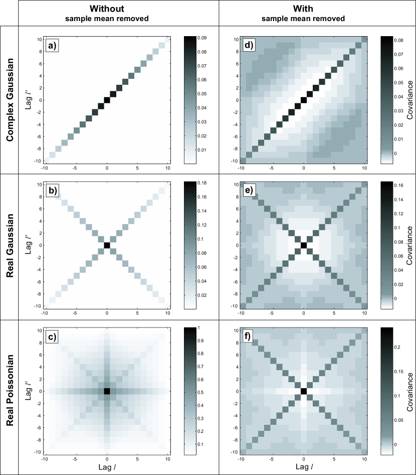
Figure 1: Covariance and variance between any two lags $l$ and $l^{\prime}$ of the correlogram estimator ($N=11$) with and without sample mean removal for various types of white noise signals. The first column of panels, namely a), b) and c), are the correlogram without sample mean removal, $\widehat{R}^{(\mu)}[l]$, defined in equation (1); while the second column of panels, namely d), e) and f), are the correlogram with sample mean removal, $\widehat{C}^{(\overline{\mu})}[l]$, defined in equation (5). The signal in the first row of panels, namely a) and d) is analytic Gaussian white noise $\sigma^{2}=1$; the second row, b) and e), is real Gaussian white noise; the third row, c) and f), is real Poissonian white noise with $\mu=1$. In all plots, the variance is along the $l=l^{\prime}$ diagonal while the rest, $l\neq l^{\prime}$ is strictly covariance. Note that the gray-scale in the second column is different from the linear scale of the first column in order to enhance the structure of the covariance.

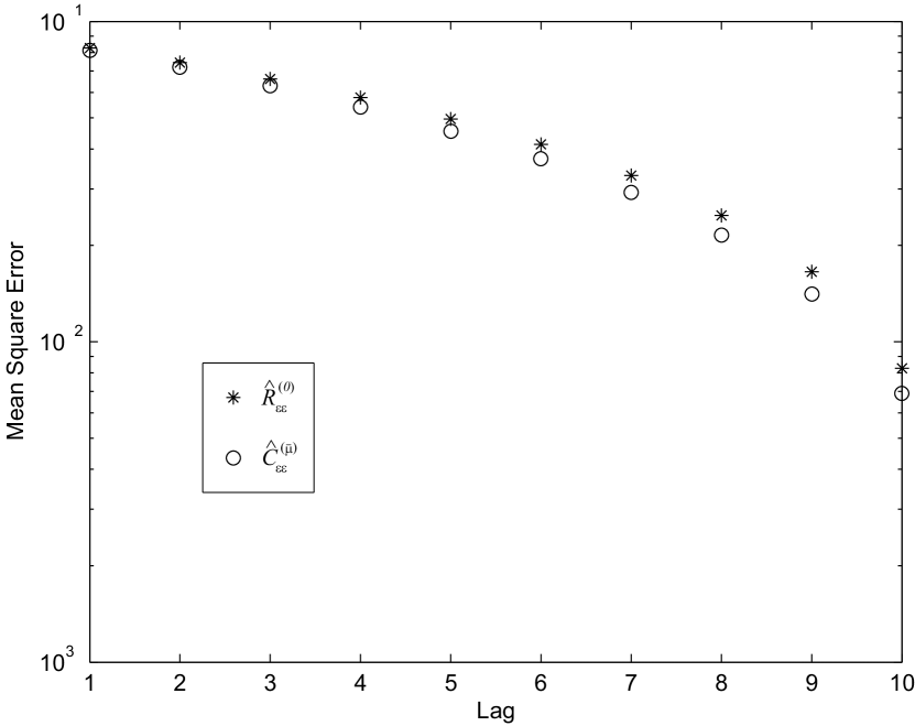
Figure 2: Comparison of the MSE of the $\widehat{R}^{(0)}$and $\widehat{C}^{(\overline{\mu})}$estimators with $\mathcal{W}_{P}[l]$ weights for the case of analytic Gaussian white noise with $\sigma^{2}=1$. For all lags, the autocovariance sequence estimator using the sample mean, i.e. $\widehat{C}^{(\overline{\mu})}$represented by circles, exhibits a smaller MSE than the estimator using the known mean, i.e. $\widehat{R}^{(0)}$ represented by stars.

5.1 $\widehat{R}^{(0)}$and $\widehat{C}^{(\overline{\mu})}$ as autocovariance estimators when mean is known

In the preceding sections we have assumed that the mean of the data sequence we are trying to estimate the autocovariance of is unknown. What can be said if the mean is known? It would seem natural that if we knew the mean we would subtract it from the data samples and use the estimator $\widehat{R}^{(0)}$. Thus we would not use the estimator $\widehat{C}^{(\overline{\mu})}$ as it involves estimation of the mean which we already know. Surprisingly however, inspection of the sampling properties presented here show that this choice of estimators is not immediately obvious.

The MSE of the estimator $\widehat{C}^{(\overline{\mu})}$ is, in fact, smaller than that of the estimator $\widehat{R}^{(0)}$ for general white noise, assuming the same lag window is used in both estimators. The difference in the MSE is

$$2\sigma^{4}\frac{l}{N^{2}}(N-l)\mathcal{W}^{2}[l]$$ (26)

and is plotted in Figure 2. This difference tends asymptotically to zero as $N$ is increased, but for finite sample sizes the $\widehat{C}^{(\overline{\mu})}$ is always better than the $\widehat{R}^{(0)}$ in the MSE sense. This is counter-intuitive as it seems to violate the principle that the more one knows about something, the better one can estimate it.

The solution to this conundrum is that although the error in the covariance estimate is smaller, the error in the estimate of the mean is on the other hand larger. Specifically the difference in the MSE in the mean estimate is $\sigma^{4}/N$. If take, e.g., the weights $\mathcal{W}_{P}[l]$ and use the inequality $l<N$ then the MSE for lag $l$ must be smaller than $2\sigma^{4}l/N^{3}$ and so the total MSE of the estimator is of the order $\sigma^{4}/N$. This is comparable to the MSE in the sample mean. Thus the total error, autocovariance and mean estimation, is not better for the $\widehat{C}^{(\overline{\mu})}$ compared with $\widehat{R}^{(0)}$.

Furthermore $\widehat{C}^{(\overline{\mu})}$ has a nonzero covariance between its lag estimates which $\widehat{R}^{(0)}$does not have. This can be understood from the following observation: that the sum over all non-negative lags of the estimator $\widehat{R}^{(\mu)}$ with periodogram weighting is equal to sample size times the square of the sample mean, i.e.

$${\displaystyle\sum_{l=0}^{N-1}}\widehat{R}_{zz}^{(P)}[l]=\frac{1}{N}{\displaystyle\sum_{l=0}^{N-1}}\sum_{k=1}^{N-l}z^{*}[k]z[k+l]=N\left|\sum_{k=1}^{N-1}z[k]\right|^{2}=N\left|\overline{z}\right|^{2}$$

for any process $\{z[k]\}$. See [8] for further discussions. This shows that $\widehat{R}_{zz}^{(P)}$ and the sample mean $\overline{z}$ are related. But since $\widehat{C}^{(\overline{\mu})}$ is based on $\widehat{R}_{zz}^{(P)}$ and $\overline{z}$ enters into every lag estimate, this suggests that there is an interdependence between lags and explain the nonzero covariance of the lags.

5.2 When to use the sample mean if the mean is assumed small

Let us now look at the situation when we believe that the mean is small. The question is which estimator is better: the one without or the one with sample mean removal. If we use the former we run the risk that the error in the estimated mean is large than the true mean. On the other hand, the mean may not be exactly zero so the latter estimate will also be off. There is a trade off here and we wish to find a criterion for when the sample mean should be removed.

Inspection of the results presented earlier suggest that as a rule of thumb the two estimators are roughly equal when

$$|\mu|=\frac{\sigma}{\sqrt{2N}}$$ (27)

and when $|\mu|<\sigma/\sqrt{2N}$ , $\widehat{R}^{(\mu)}$ is preferable to $\widehat{C}^{(\overline{\mu})}$ and when $|\mu|>\sigma/\sqrt{2N}$, $\widehat{C}^{(\overline{\mu})}$ is preferable to $\widehat{R}^{(\mu)}$. This condition can be understood in an intuitive way as follows. The sample mean is an estimate of the population mean with a relative error of $(\sigma/\sqrt{N})/|\mu|$. It makes sense to use this estimate in the correlogram instead of the unknown mean only if this relative error is smaller than 1, i.e. when $|\mu|>\sigma/\sqrt{2N}$. This is because the absolute error if we do not remove anything is of course only $|\mu|$. Thus we arrive at the condition as the found above (27).

Naturally, if we do not know the mean we will not be able asses the equality (27) exactly, but one could instead get it approximately by using the sample mean and the sample variance of the given data samples.

6 Conclusion

We have presented expressions for the bias, variance, covariance, mean-square error of the classical correlogram estimator with and without sample mean estimation for general complex white noise with arbitrary mean. A summary of the sampling properties of the estimators for $\epsilon[\cdot]$, i.e., complex higher order white noise with arbitrary mean is as follows. The second-order sampling properties of the correlogram without sample mean removal, $\widehat{R}^{(\mu)}$, are in summary:

• $\epsilon[\cdot]$ moment dependence: cumulants up to fourth order $\{\mu,\sigma^{2},s^{2},\kappa_{3},\kappa_{4}\}$

• Bias: unbiased for $1/(N-l)$ weighting, even when $\mu\neq 0$

• Covariance: piecewise linear lag dependent covariance before weighting

• Mean square error: is asymptotically proportional to $|\mu|^{4}$ when $\mu\neq 0$ while if $\mu=0$ the MSE is asymptotically equal to $\sigma^{4}(N-|l|)\mathcal{W}^{2}[l]$

For the correlogram with sample mean removal, $\widehat{C}^{(\overline{\mu})}$, a summary of second-order sampling properties is:

• $\epsilon[\cdot]$ moment dependence: only even order cumulants $\{\sigma^{2},s^{2},\kappa_{4}\}$

• Bias: nonzero lags biased for all weighting functions, zero lag unbiased for $\mathcal{W}[0]=1/(N-1)$

• Covariance: piecewise quadratic lag dependent covariance before weighting

• Mean square error: asymptotically equal to $\sigma^{4}(N-|l|)\mathcal{W}^{2}[l]$

In terms of the properties of the process, we have found that a nonzero mean can lead to covariance between lags of the correlogram, and that complex valued processes lift the degeneracy between positive and positive lags, (that is that the sampling properties of positive lags and negative lags are different), and distinguishes between analytic and non-analytic processes.

For both estimators, the both the variance and the covariance are in general lag dependent. We conclude therefore that neither $\widehat{R}^{(\mu)}$ nor $\widehat{C}^{(\overline{\mu})}$ with the standard lag weights $\mathcal{W}_{U}[l]$ and $\mathcal{W}_{P}[l]$ are optimal for estimating the autocorrelation/autocovariance of noise processes with an unknown mean.

Finally, we found that the sampling properties suggest that one should always remove the mean if it is known apriori. If the mean is not known, the sample mean should be removed only when $|\mu|>\sigma/\sqrt{2N}$, i.e. $\widehat{R}_{\epsilon\epsilon}^{(\mu)}$ is preferable to $\widehat{C}_{\epsilon\epsilon}^{(\overline{\mu})}$ if $|\mu|<\sigma/\sqrt{2N}$.

References

- [1] T. W. Anderson. The Statistical Analysis of Time Series. John Wiley & Sons, Inc., 1971.
- [2] M. S. Bartlett. On the theoretical specification and sampling properties of autocorrelated time-series. Supplement to the Journal of the Royal Statistical Society, 8(1):27–41, 1946.
- [3] Juilus S. Bendat and Allan G. Piersol. Random data: analysis and measurement procedures. John Wiley and Sons, Inc, third edition edition, 2000.
- [4] T. D. Carozzi and A. M. Buckley. Deriving the sampling errors of correlograms for general white noise. To be published in Biometrika, 2005, arXiv:physics/0505145.
- [5] Gwilym M. Jenkins and Donald G. Watts. Spectral Analysis and its applications. Holden-Day, Inc, 1968.
- [6] F. H. C. Marriott and J. A. Pope. Bias in the estimation of autocorrelations. Biometrika, 41(3/4):390–402, 1954.
- [7] Chrysostomos L. Nikias and Jerry M. Mendel. Signal processing with higher-order spectra. IEEE Signal Processing Magazine, 10(3):10–37, July 1993.
- [8] Donald B. Percival. Three curious properties of the sample variance and autocovariance for stationary processes with unknown mean. The American Statistician, 47(4):274–276, 1993.