Is There a Real-Estate Bubble in the US?

Abstract

We analyze the quarterly average sale prices of new houses sold in the USA as a whole, in the northeast, midwest, south, and west of the USA, in each of the 50 states and the District of Columbia of the USA, to determine whether they have grown faster-than-exponential which we take as the diagnostic of a bubble. We find that 22 states (mostly Northeast and West) exhibit clear-cut signatures of a fast growing bubble. From the analysis of the S&P 500 Home Index, we conclude that the turning point of the bubble will probably occur around mid-2006.

,

1 Is there a real-estate bubble in the US? Lessons from the past UK bubble

In the aftermath of the burst of the “new economy” bubble in 2000, the Federal Reserve aggressively reduced short-term rate yields in less than two years from 6^1/2 % to 1 % in June 2003 in an attempt to coax forth a stronger recovery of the US economy. In March 2003, we released a paper published a few months later [13] addressing the growing apprehension at the time (see for instance [1]) that this loosening of the US monetary policy could lead to a new bubble in real estate, as strong housing demand was being fueled by historically low mortgage rates. As of March 2003, we concluded that, “while there is undoubtedly a strong growth rate, there is no evidence of a super-exponential growth in the latest six years,” giving “ no evidence whatsoever of a bubble in the US real estate market” [13].

More than two years have passed. During that period, the historically low Fed rate of 1% remained stable from June 2003 to June 2004. Since June 2004, the Fed (specifically, the Federal Open Market Committee (FOMC)) has increased its discount rate by increments of 0.25% at each of its successive meetings (the FOMC holds 8 meetings per year): at the time of writing (end of May 2005), the last 0.25% increase occurred on May 3rd, 2005 to yield a short-term rate of 3%, the next meeting of the FOMC being scheduled on 29/30 June 2005 . While the short-term interest rates are following a steady upward trend of 2% per year since June 2004, long-term rates have not followed, some going down while other long-term rates increasing only slightly. Thus, long-term mortgage interest rates have remained extremely low by historical standard. The Office of Federal Housing Enterprise Oversight (OFHEO), the government unit tasked with regulating Fannie Mae and Freddie Mac , recently published a research paper stating that “The housing market achieved record levels of activity and contributed significantly to the economic recovery … Falling mortgage rates stimulated housing starts and sales, and many refinancing borrowers took out loans that were larger than those they paid off, providing additional funds for consumption expenditures… According to Freddie Mac, homeowners who refinanced in 2003 converted almost $139 billion in home equity into cash, up from $105 billion in 2002.” This has led to renewed worries that a real-estate bubble is on its way.

The purpose of this paper is to revisit this question, using the more than two additional years of data since our previous analysis [13]. As explained in our previous paper on real-estate bubbles [13], our analysis relies on a general theory of financial crashes and of stock market instabilities developed in a series of works (see [9, 3, 5, 2, 8, 6] and references therein). The main ingredient of the theory is the existence of positive feedbacks in stock markets as well as in the economy. Positive feedbacks, i.e., self-reinforcement, refer to the fact that, conditioned on the observation that the market has recently moved up (respectively down), this makes it more probable to keep it moving up (respectively down), so that a large cumulative move may ensue. The concept of “positive feedbacks” has a long history in economics. It can occur for instance in the form of “increasing returns”– which says that goods become cheaper the more of them are produced (and the closely related idea that some products, like fax machines, become more useful the more people use them). Positive feedbacks, when unchecked, can produce runaways until the deviation from equilibrium is so large that other effects can be abruptly triggered and lead to rupture or crashes. Alternatively, it can give prolonged depressive bearish markets. There are many mechanisms leading to positive feedbacks including investors’ over-confidence, imitative behavior and herding between investors, refinancing releasing new cash re-invested in houses, lower requirement margins due to uprising prices, and so on. Such positive feedbacks provide the fuel for the development of speculative bubbles, by the mechanism of cooperativity, that is, the interactions and imitation between investors may lead to collective behaviors similar to crowd phenomena. Different types of collective regimes are separated by so-called critical points which, in physics, are widely considered to be one of the most interesting properties of complex systems. A system goes critical when local influences propagate over long distances and the average state of the system becomes exquisitely sensitive to a small perturbation, i.e. different parts of the system become highly correlated. Another characteristic is that critical systems are self-similar across scales: at the critical point, an ocean of traders who are mostly bearish may have within it several continents of traders who are mostly bullish, each of which in turns surrounds seas of bearish traders with islands of bullish traders; the progression continues all the way down to the smallest possible scale: a single trader [12]. Intuitively speaking, critical self-similarity is why local imitation cascades through the scales into global coordination. Critical points are described in mathematical parlance as singularities associated with bifurcation and catastrophe theory. At critical points, scale invariance holds and its signature is the power law behavior of observables.

Mathematically, these ideas are captured by the power law

$$\ln[p(t)]=A+B(t_{c}-t)^{m}~{},$$ (1)

where $p(t)$ is the house price or index, $t_{c}$ is an estimate of the end of a bubble so that $t<t_{c}$ and $A,B,m$ are coefficients. If the exponent $m$ is negative, $\ln[p(t)]$ is singular when $t\to t_{c}^{-}$ and $B>0$ ensuring that $\ln[p(t)]$ increases. If $0<m<1$, $\ln[p(t)]$ is finite but its first derivative $d\ln[p(t)]/dt$ is singular at $t_{c}$ and $B<0$ ensuring that $\ln[p(t)]$ increases. Extension of this power law (1) takes the form of log-periodic power law (LPPL) for the logarithm of the price

$$\ln[p(t)]=A+B(t_{c}-t)^{m}+C(t_{c}-t)^{m}\cos\left[\omega\log(t_{c}-t)-\phi\right],$$ (2)

where $\phi$ is a phase constant and $\omega$ is the angular log-frequency. This first version (2) amounts to assume that the potential correction or crash at the end of the bubble is proportional to the total price [3]. In contrast, a second version assumes that the potential correction or crash at the end of the bubble is proportional to the bubble part of the total price, that is to the total price minus the fundamental price [3]. This gives the following price evolution:

$$p(t)=A+B(t_{c}-t)^{m}+C(t_{c}-t)^{m}\cos\left[\omega\log(t_{c}-t)-\phi\right]~{}.$$ (3)

As explained in [13, 6], we diagnose a bubble using these models by demonstrating a faster-than-exponential increase of $p(t)$, possibly decorated by log-periodic oscillations.

Before presenting the result of our analysis using these models on the US real-estate bubble, it is appropriate to discuss how our detection of a bubble in the UK real-estate market fared since March 2003. In [13], we reported “unmistakable signatures (log-periodicity and power law super-exponential acceleration) of a strong unsustainable bubble” for the UK real-estate market. We identified two potential turning points in the UK bubble reported in Tables 2 and 3 of [13]: end of 2003 and mid-2004. The former (resp. later) was based on the use of formula (2) (resp. (3)). These predictions were performed in Feb. 2003 (again our paper was released in early March 2003 on an electronic archive ). We stress that these turning points can be either crashes or changes of regimes according to the theory coupling rational expectation bubbles with collective herding behavior described in [2, 5, 11, 4]. In other words, the theory describes bubbles and their end but not the crash itself: the end of a bubble is the most probable time for a crash, but a crash can occur earlier (with low probability) or not at all; the possibility that no crash occurs is necessary for the bubble to exist, otherwise, rational investors would anticipate the crash and, by backward reasoning, would make it impossible to develop.

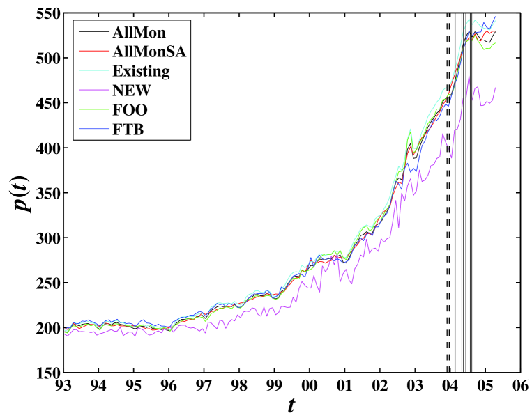
Figure 1: Plot of the UK Halifax house price indices from 1993 to April 2005 (the latest available quote at the time of writing). The two groups of vertical lines correspond to the two predicted turning points reported in Tables 2 and 3 of [13]: end of 2003 and mid-2004. The former (resp. later) was based on the use of formula (2) (resp. (3)). These predictions were performed in Feb, 2003.

Figure 1 plots the UK Halifax house price index (HPI) from 1993 to April 2005 (the latest available quote at the time of writing). The two groups of vertical lines correspond to the two predicted turning points mentioned above. The first set of predicted turning points (dashed lines in Figure 1) anticipated by half-a-year the turning point which occurred mid-2004 as predicted by the second set.

Our analysis presented below uses three data sets: (1) the regional data (Northeast, Midwest, west, south and USA as a whole) of the quarterly average sale prices of new houses up to the fourth quarter of 2004 (the latest data available); (2) the house price index of individual states (50 states $+$ DC), up to Q1 of 2005, quarterly data; and (3) daily data of the S&P 500 Home Index, up to May 6, 2005. We first present in section 2 a broad-brush analysis using the exponential versus power law models of house price appreciation for the whole continental US and then by regions. We then turn to a state-by-state analysis which leads to a partition into three classes: (i) non-bubbling states, (ii) recent-bubbling states and (iii) clearly-bubbling states. For the states for which a bubble seems to be clearly established according to our criterion, we provide a first estimation of the critical time of the end of the bubble. We then turn to the more elaborate LPPL models (2) and (3) and a nonlinear extension, using the daily data of the S&P 500 Home Index up to May 6, 2005.

2 Evidence of a US real-estate bubble by faster-than-exponential growth

Figures 2 show the quarterly average sale prices of new houses sold in all the states of the USA as well as in the four main regions, Northeast, Midwest, South and West, from 1993 to the fourth quarter of 2004 as a function of time $t$. The smooth curve is the power-law fit (1) to the data. Except for the midwest and south regions, one can observe a strong upward curvature in these linear-logarithmic plots, which characterize a faster-than-exponential price growth (recall that an exponential growth would qualify as a straight line in such linear-logarithmic plots). The existence of a strong upward curvature characterizing a faster-than-exponential growth is quantified by the relatively small values of the exponent $m$ ($=0.55$ for all states, $=0.64$ for the Northeast region, $=0.18$ for the West region).

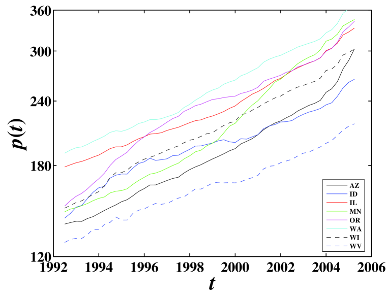
Figure 4: (Color online) Quarterly HPI in the 8 states exhibiting a recent upward acceleration following an approximately constant exponential growth rate. The corresponding states are given in the legend.

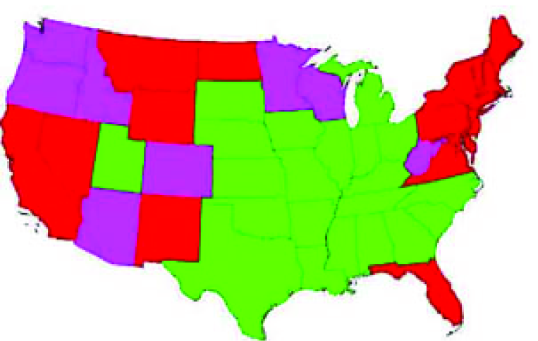
Figure 6: Geographical synopsis of the classification in three families: the first family of non-bubbling states of figure 3 in green, the second family of recently-bubbling states in figure 4 in magenta and the third family of clearly bubbling states in figure 5 in red. Hawaii and Alaska, both in red, are not drawn here.

To have a closer look, we examined quarterly data of House Price Index (HPI) for each individual state. Rather than following a formal procedure and developing sophisticated statistical tests, the obvious differences between the price trajectories in the different states led us to prefer a more intuitive approach consisting of classifying the different states according to how strongly they depart from a steady exponential growth. We found three families, shown in figures 3, 4 and 5. Figure 3 shows the quarterly HPI in the 21 states which have an approximately constant exponential growth, qualified by a linear trend in a linear-logarithmic scale. The thick straight line at the bottom of the figure is the average over all 21 states corresponding to an annual growth rate of 4.6% over the last 13 years (we did not use the data prior to 1992 to avoid contamination by the turning point of the previous bubble in 1991). Figure 4 shows the quarterly HPI in the 8 states exhibiting a recent upward acceleration following an approximately constant exponential growth rate. Figure 5 shows the quarterly HPI in the 22 states exhibiting a clear upward faster-than-exponential growth. These 22 states thus exhibit the hallmark of a real-estate bubble. Figure 6 provides a geographical synopsis of this classification in three families: the first family of figure 3 is green, the second family of figure 4 is magenta, and the third family of figure 5 is red. As often discussed by commentators, prices have accelerated mostly to the Northeast and West regions, which is consistent with Fig. 2.

Consider the third family of 22 states where we diagnose a bubble, as shown in figure 5. Can a power law fit with (1) reveal the end of the bubble? Such turning point is in principle measured by the time $t_{c}$ in expression (1), which gives the time at which the bubble should end. In order to get less noisy data, we averaged over the 22 price trajectories of figure 5 and then fitted the obtained average with (1) (with the modification that $t_{c}-t$ is replaced by $|t_{c}-t|$ to allow for a more robust estimation) over a time interval from $t_{\rm start}$ to the last available data point (2005Q1). Figure 7 shows the obtained critical time $t_{c}$ and exponent $m$ as a function of $t_{\rm start}$. Varying $t_{\rm start}$ allows us to test for sensitivity with respect to the different time periods and assess the robustness of the results. Not surprisingly, we find that the fitted $t_{c}$ is close to the last data points for some $t_{\rm start}$, a result which has been found to systematically characterize power law behaviors [6]. Therefore, the power law fit is not very reliable to determine the end of the real-estate bubble. However, the relative stability of $m$ in the range $0.1-0.5$ as a function of $t_{\rm start}$, which characterizes a faster-than-exponential growth, indicates that the simple power law (1) is already a good model.

3 Extension to the LPPL model and discussion

The previous tests performed in [9, 3, 5, 2, 8, 6] (and references therein) show that the problem with the too-large sensitivity of $t_{c}$ in the simple power law model with respect to the few last data points are alleviated by using the more sophisticated LPPL models (2) and (3). Here, we use both LPPL models (2) and (3) as well as the so-called 2nd-order Landau LPPL introduced in [7] . In a nutshell, the 2nd-order Landau LPPL extends the LPPL model by allowing for a first nonlinear correction which amounts to combining two log-frequencies $\omega_{0}$ (close to $t_{c}$) and $\omega_{\infty}$ (far from $t_{c}$).

We fit the daily data of the S&P 500 Home Index to the LPPL and 2nd-order Landau LPPL models in a time interval from $t_{\rm start}$ to the last available data point (April 2005). Figure 8 presents the dependence of $\omega$ for the LPPL model and of $\omega_{0}$ for the 2nd-order Landau LPPL model as a function of $t_{\rm start}$. We find $\omega\approx 10$ and $\omega_{0}$ oscillating between $\omega\approx 10$ and $\omega/2$, as we expect from the generic existence of harmonics (see our previous extended discussions in [10, 14]). The stability of $\omega_{0}$ and the compatibility between the two descriptions is a signature of the robustness of the signal. Figure 9 shows the predicted critical time $t_{c}$ as a function of $t_{\rm start}$ obtained from the fits with the LPPL and the 2nd-order Landau LPPL models. The large spreads of values for $t_{\rm start}$ earlier than 1993 reflects the fact that the bubble has really started only after 1993.

We observe a good stability of the predicted $t_{c}\approx$ mid-2006 for the two LPPL models (2) and (3). The spread of $t_{c}$ is larger for the second-order LPPL fits but brackets mid-2006. As mentioned before, the power law fits are not reliable. We conclude that the turning point of the bubble will probably occur around mid-2006.

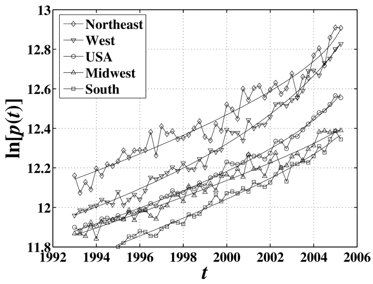
Figure 2: Quarterly average sale prices of new houses sold in all the states of the USA and by regions (Northeast, Midwest, South and West) from 1993 to the first quarter of 2005 as a function of time $t$. The smooth lines are the power-law fits (1) to the five data sets. The values of fitted parameters for the West are $t_{c}=2008.3$, $m=0.18$, $A=15.48$, and $B=-2.16$ with the r.m.s. of the fit residuals being 0.0275. The values of the fitted parameters for USA are $t_{c}=2006.0$, $m=0.55$, $A=12.75$, and $B=-0.212$ with the r.m.s. of the fit residuals being 0.0174. The values of fitted parameters for the Northeast are $t_{c}=2005.2$, $m=0.64$, $A=12.92$, and $B=-0.154$ with the r.m.s. of the fit residuals being 0.0485. The values of fitted parameters for the South are $t_{c}=2005.2$, $m=0.78$, $A=12.37$, and $B=-0.092$ with the r.m.s. of the fit residuals being 0.0215. The values of fitted parameters for the Midwest are $t_{c}=2005.2$, $m=0.84$, $A=12.40$, and $B=-0.066$ with the r.m.s. of the fit residuals being 0.0308.

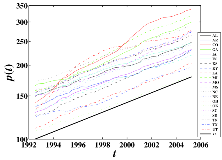
Figure 3: (Color online) Quarterly HPI in the 21 states which have an approximately constant exponential growth, qualified by a linear trend in a linear-logarithmic scale. The thick straight line at the bottom of the figure is the average over all 21 states corresponding to an annual growth rate of 4.6% over the last 13 years. The corresponding states are given in the legend. Note that Colorado seems to be on a faster trend.

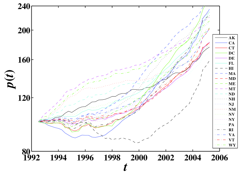
Figure 5: (Color online) Quarterly average HPI in the 21 states and in the District of Columbia (DC) exhibiting a clear upward faster-than-exponential growth. For better representation, we have normalized the house price indices for the second quarter of 1992 to 100 in all 22 cases. The corresponding states are given in the legend.

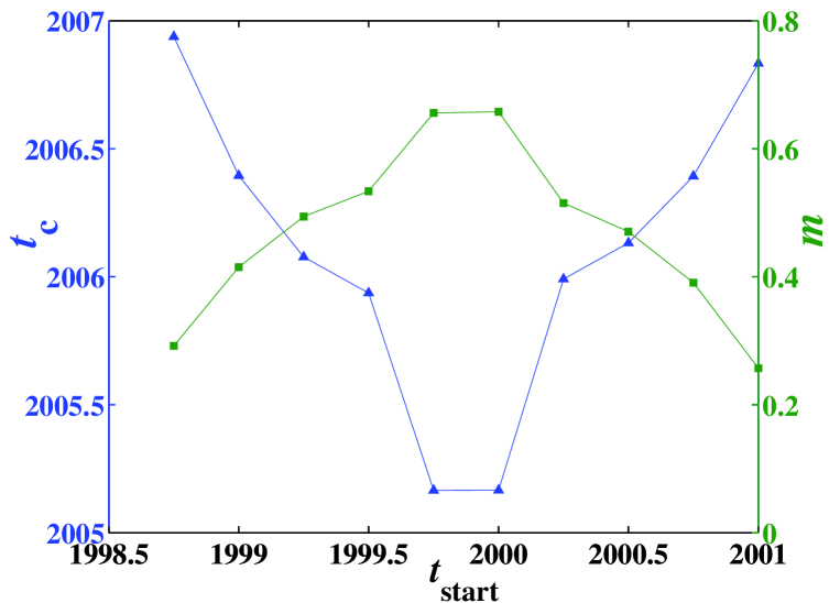
Figure 7: Critical time $t_{c}$ and exponent $m$ as a function of $t_{\rm start}$, obtained by fitting with the power law (1) (with the modification that $t_{c}-t$ is replaced by $|t_{c}-t|$ to allow for a more robust estimation) the price trajectory obtained by averaging over the 22 states of figure 5.

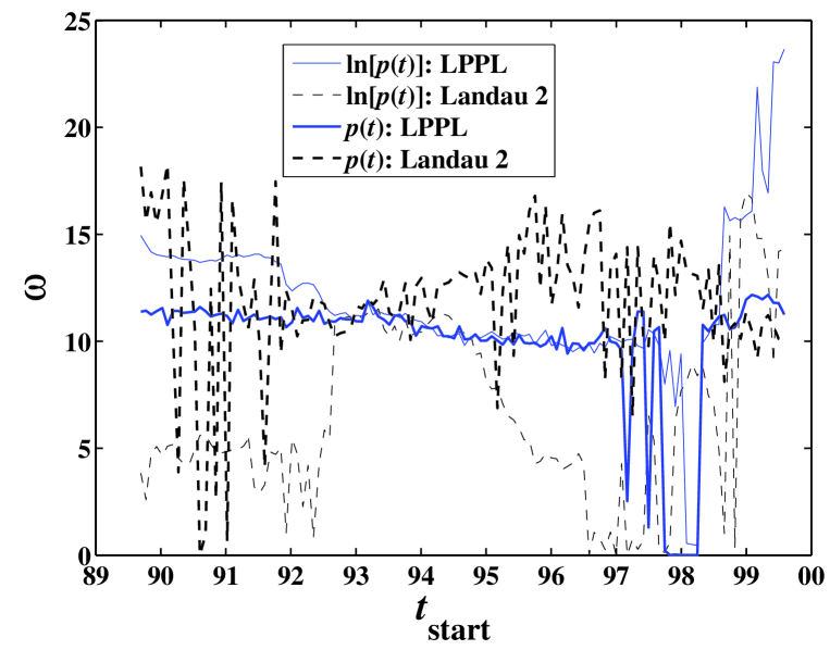
Figure 8: Dependence of $\omega$ for the LPPL model and of $\omega_{0}$ for the 2nd-order Landau LPPL model as a function of $t_{\rm start}$ obtained by fitting the S&P 500 Home Index up to May 6, 2005.

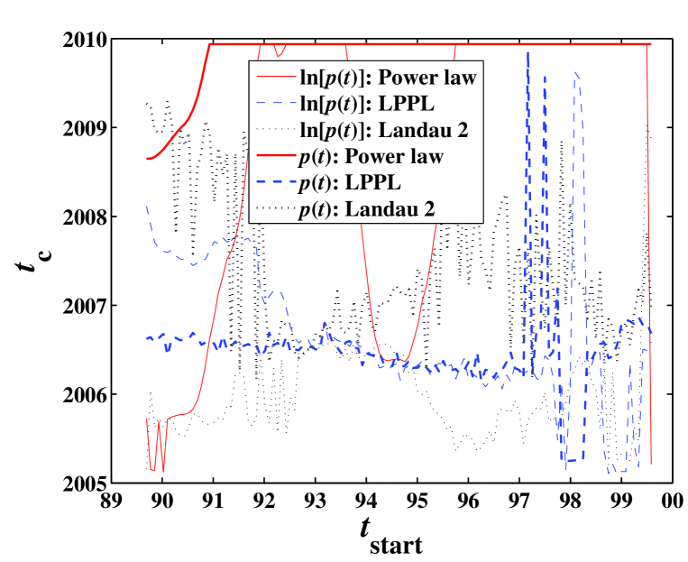
Figure 9: Predicted critical time $t_{c}$ as a function of $t_{\rm start}$ obtained from the fits with the LPPL and the 2nd-order Landau LPPL models as in figure 8.

References

- [1] House of cards, The Economist, May 29, 2003.
- [2] A. Johansen, O. Ledoit and D. Sornette, Crashes as critical points, International Journal of Theoretical and Applied Finance 3 (2), 219-255 (2000).
- [3] A. Johansen and D. Sornette, Critical crashes, Risk, Vol 12, No. 1, p.91-94 (1999).
- [4] A. Johansen and D. Sornette, Endogenous versus exogenous crashes in financial markets, in press in “Contemporary Issues in International Finance” (Nova Science Publishers, 2005) (http://arXiv.org/abs/cond-mat/0210509)
- [5] A. Johansen, D. Sornette and O. Ledoit, Predicting financial crashes using discrete scale invariance, Journal of Risk 1 (4), 5-32 (1999)
- [6] D. Sornette, Why Stock Markets Crash (Critical Events in Complex Financial Systems), Princeton University Press, Princeton, NJ, 2002.
- [7] D. Sornette and A. Johansen, Large financial crashes, Physica A 245, N3-4, 411-422 (1997).
- [8] D. Sornette and A. Johansen, Significance of log-periodic precursors to financial crashes, Quantitative Finance 1, 452-471 (2001).
- [9] D. Sornette, A. Johansen and J.-P. Bouchaud, Stock market crashes, precursors and replicas, J. Phys. I France 6, 167-175 (1996).
- [10] D. Sornette and W.-X. Zhou, The US 2000-2002 market descent: how much longer and deeper? Quantitative Finance 2, 468-481 (2002).
- [11] D. Sornette and W.-X. Zhou, Predictability of large future changes in major financial indices, in press in the International Journal of Forecasting (2005) (http://arXiv.org/abs/cond-mat/0304601)
- [12] K. G. Wilson, Problems in Physics with many scales of length, Scientific American 241, 158-179 (1979).
- [13] W.-X. Zhou and D. Sornette, 2000-2003 real estate bubble in the UK but not in the USA, Physica A 329, 249-263 (2003).
- [14] W.-X. Zhou and D. Sornette, Renormalization group analysis of the 2000-2002 anti-bubble in the US S&P 500 index: Explanation of the hierarchy of 5 crashes and prediction, Physica A 330, 584-604 (2003).