Parametric Autoresonance in Faraday waves

Abstract

We develop a theory of parametric excitation of weakly nonlinear standing gravity waves in a tank, which is under vertical vibrations with a slowly time-dependent (“chirped”) vibration frequency. We show that, by using a negative chirp, one can excite a steadily growing wave via parametric autoresonance. The method of averaging is employed to derive the governing equations for the primary mode. These equations are solved analytically and numerically, for typical initial conditions, for both inviscid and weakly viscous fluids. It is shown that, when passing through resonance, capture into resonance always occurs when the chirp rate is sufficiently small. The critical chirp rate, above which breakdown of autoresonance occurs, is found for different initial conditions. The autoresonance excitation is expected to terminate at large amplitudes, when the underlying constant-frequency system ceases to exhibit a non-trivial stable fixed point.

I Introduction

There are two ways of driving a classical nonlinear oscillator by a small oscillating force: via either external or parametric resonance. In both cases, the initial growth of the amplitude of the oscillator is arrested, even without dissipation, when nonlinear effects come into play. This is due to the fact that the natural frequency of a nonlinear oscillator is amplitude-dependent, so a mismatch between the (invariable) driving frequency and the natural frequency appears Landau1 .

To overcome the nonlinear mismatch and maintain phase locking between the driving force and the oscillator, one can slowly vary the driving frequency with time so as to achieve a persistent growth of the oscillations. This simple and versatile method is called autoresonance: either external, or parametric. To emphasize the difference between the two, let us watch a child on a swing. When a parent pushes the swing (once in each cycle), he gradually increases the time interval between the pushes as the swing amplitude grows. Here he employs external autoresonance. On the contrary, when the child swings himself (he achieves it by moving the position of his center of mass up and down twice in each cycle), he gradually increases the period of these modulations as the swing amplitude grows. This is parametric autoresonance.

The simple model of a nonlinear oscillator, excited via external autoresonance, has found numerous applications in physics, see e.g. Ref. Friedland1 for a brief review. The external autoresonance scheme has been also generalized to systems with an infinite number of degrees of freedom, such as nonlinear waves Meerson5 ; Meerson3 ; Lazar_3wave and vortices vortices . In contrast to the external autoresonance, parametric autoresonance has received much less attention Khain . In this work we generalize to nonlinear waves the theory, developed in Ref. Khain for a nonlinear oscillator. Specifically, we show that the parametric autoresonance mechanism can be used for driving nonlinear standing gravity waves with a steadily growing amplitude on a free surface of a fluid.

Michael Faraday Faraday was the first to observe that, when a tank containing a fluid is periodically vibrated in the vertical direction, a standing wave pattern forms at the free surface of the fluid when the vibration frequency is twice the frequency of the surface vibrations. This phenomenon is a classic example of parametric resonance, because the vertical acceleration of the tank - an intrinsic parameter of the system - depends on time via the periodic vibration. Lord Rayleigh Rayleigh carried out a further series of experiments, which supported Faraday’s observations, and also developed a linear theory for these waves in terms of a linear Mathieu equation. Benjamin and Ursell Ursell advanced the linear theory further. Subsequently, Miles Miles1 ; Miles2 ; Miles3 , Douady douady , Milner milner , and Decent and Craik decent formulated a weakly nonlinear theory based on amplitude expansion, while some of these and indeed numerous other works dealt with experimental studies of Faraday waves.

Being interested in parametric autoresonance, we add a new dimension to the problem of Faraday waves and investigate weakly nonlinear standing gravity waves formed when the vibration frequency is slowly decreased (chirped downwards) in time. We show that the negative frequency chirp causes a persistent growth of the wave amplitude. Like in other instances of autoresonance, the exact form of the frequency chirp is unimportant once the chirp sign is correct, and the chirp rate is not too high. The autoresonance excitation is expected to terminate at large amplitudes, when an underlying dynamical system, corresponding to the case of a constant frequency, ceases to exhibit a non-trivial stable fixed point.

Here is the layout of the rest of the paper. Section II presents a brief overview of theory of weakly nonlinear Faraday waves with a constant driving frequency. Sections III and IV deal with theory of chirped Faraday waves, in inviscid (Sec. III) and low-viscosity (Sec. IV) fluids. Section V presents a brief discussion of our results.

II Weakly nonlinear Faraday waves

II.1 Inviscid fluid

To set the stage for a theory of chirped Faraday waves, we need to briefly review the theory of weakly nonlinear Faraday waves with a constant driving frequency. Consider a quasi-two-dimensional rectangular tank with a fluid of length $l$, width $w$ and depth $h$, so that $l\gg w$. We assume that the elevation of the fluid, caused by the wave, depends only on the longitudinal coordinate $x$ and time $t$, so that we have a quasi-two-dimensional flow in the $xz$ plane ($z$ is the vertical coordinate). The unperturbed level of the fluid is at $z=0$. The vertical displacement of the vibrating tank is described by the equation

$$\zeta(t)=a_{0}\cos(2\omega\,t)\,.$$ (1)

We assume weak forcing, that is the vibration acceleration is much less than the gravity acceleration $g$, and introduce a small dimensionless parameter $\varepsilon$:

$$\varepsilon=\frac{\omega^{2}a_{0}}{g}\ll\,1\,.$$ (2)

In the limit of inviscid fluid the flow remains potential once it is potential at $t=0$, and the external forces are potential Lamb , as is the case here. The assumption of a potential flow is also approximately valid in a low-viscosity fluid Ursell . We also assume that the wavelength of the standing wave is much larger than the capillary length of the fluid and neglect the capillary effects throughout the paper. The linear dispersion relation for the wave is $\omega_{n}^{2}=\,gk_{n}\tanh(k_{n}h)$, where $\omega_{n}$ is the natural frequency of the $n$-th mode, $k_{n}=2\pi/\lambda_{n}=n\pi/l$ is the wave number of the $n$-th mode, and $n=1,2,\dots$.

The governing equations for the velocity potential $\varphi(x,z,t)$ and the wave profile $\eta(x,t)$ are Ursell ; Lamb ; Landau2 ; Currie :

$$\nabla^{2}\varphi = 0\,,$$ (3)

$$\left.\left[\varphi_{t}+\frac{1}{2}(\varphi_{x}^{2}+\varphi_{z}^{2})+(g+\ddot{\zeta})\eta\right]\right|_{{}_{z=\eta}} = 0\,,$$ (4)

$$\left(\eta_{t}+\varphi_{x}\eta_{x}-\varphi_{z}\right)|_{{}_{z=\eta}} = 0\,,$$ (5)

$$\varphi_{z}\,|_{{}_{z=-h}} = 0\,,$$ (6)

where indices denote partial derivatives. The Laplace’s equation (3) describes a potential flow of an incompressible fluid. Equations (4) and (5) are the Navier-Stokes equation and the kinematic boundary condition, respectively, evaluated at the free surface. Finally, Eq. (6) is the boundary condition for the vertical velocity component at the bottom of the tank.

Let the vibration frequency be close to twice the natural frequency of the primary mode $n=1$, i.e. $\omega\simeq\omega_{1}$, so that this mode is excited via parametric resonance. In a weakly nonlinear regime it suffices to account for the excitation of only one higher order mode: the secondary mode $n=2$, which is enslaved to the primary mode Miles2 . Therefore, one should look for $\varphi(x,z,t)$ and $\eta(x,t)$ in Eqs. (3)-(6) in the following form Miles1 ; Miles2 :

$$\varphi(x,z,t)\! = \!\varphi_{0}(t)\!+\!\varphi_{1}(t)\psi_{1}(x)\frac{\cosh\left[k_{1}(z\!+\!h)\right]}{\cosh(k_{1}h)}+$$

$$+ \varphi_{2}(t)\psi_{2}(x)\frac{\cosh\left[k_{2}(z\!+\!h)\right]}{\cosh(k_{2}h)}+\dots\,,$$

$$\eta(x,t)\! = \!\eta_{1}(t)\psi_{1}(x)+\eta_{2}(t)\psi_{2}(x)+\dots\,,$$ (7)

where the eigenfunctions $\psi_{n}(x)=\sqrt{2}\,\cos\,(k_{n}x)$. The higher order terms will be neglected in the following. In the deep-water limit $k_{n}h\gg 1$, the linear dispersion relation for the wave becomes $\omega_{n}^{2}\simeq\,gk_{n}$. For this approximation to hold with an error less than 0.5%, it suffices to demand that $h>l$.

The perturbation theory we are using employs the smallness of $\varepsilon$. As will be seen later, this smallness implies a smallness of the wave amplitude compared with the wavelength, so that the dimensionless parameter $\kappa=k_{1}\eta$ is small. Expanding $\varphi(x,z=\eta,t)$ in the vicinity of the unperturbed surface $z=0$ in a power series in $\kappa$, and substituting it and the second of Eqs. (II.1) into Eqs. (4) and (5), we obtain in the leading and sub-leading orders of $\kappa$:

$$\eta_{2}(t)\simeq\frac{k_{1}\eta_{1}^{2}(t)}{\sqrt{2}}\,,$$ (8)

$$\varphi_{0}(t)\simeq-\dot{\eta}_{1}\eta_{1}\,,\;\;\varphi_{1}(t)\simeq\frac{\dot{\eta}_{1}}{k_{1}}\,,\;\;\varphi_{2}(t)\simeq 0\,.$$ (9)

As we see, the next-order corrections $\varphi_{0}$ and $\eta_{2}$ are enslaved to the primary mode, and their magnitudes are ${\cal O}(\kappa\eta_{1})$. In addition, we obtain a nonlinear differential equation of the second-order for the time-dependent amplitude of the primary mode $\eta_{1}(t)$:

$$\ddot{\eta}_{1}+\frac{1}{2}k_{1}^{2}(5\dot{\eta}_{1}^{2}\eta_{1}-3\omega_{1}^{2}\eta_{1}^{3})+\omega_{1}^{2}\left[1+4\varepsilon\cos(2\omega\,t)\right]\eta_{1}=0\,,$$ (10)

where we have used Eq. (1) and kept terms up to ${\cal O}(\kappa^{3})$. Equation (10) is a generalization of the linear Mathieu equation Bogoliubov .

Now we employ the method of averaging Bogoliubov . We make an Ansatz $\eta_{1}(t)=A_{1}(t)\cos\left[\omega_{1}t+\phi_{1}(t)\right]$ and $\dot{\eta}_{1}(t)=-\omega_{1}A_{1}(t)\sin\left[\omega_{1}t+\phi_{1}(t)\right]$ in Eq. (10) and treat the amplitude $A_{1}(t)$ and phase $\phi_{1}(t)$ as slow functions of time. (Being interested in the first-order equations with respect to $\varepsilon$, one can omit higher temporal harmonics in $\eta_{1}(t)$ Bogoliubov ; perturbative .) Let $\delta\!=\!\omega_{1}\!-\!\omega\,$ be the (small) detuning from the exact linear resonance. Then, for $\varepsilon\ll\,1$ and $|\delta|\ll\omega_{1}$, we can perform averaging over the fast time $\sim\omega_{1}^{-1}$ Bogoliubov . Introducing a new phase variable $\phi=\delta\cdot\,\!t+\phi_{1}$, we obtain:

$$\dot{A_{1}} = \varepsilon\omega_{1}A_{1}\sin(2\phi)\,,$$

$$\dot{\phi} = \varepsilon\omega_{1}\cos(2\phi)-\frac{k_{1}^{2}A_{1}^{2}\omega_{1}}{4}+\delta\,.$$ (11)

The second term in the right side of the equation for $\dot{\phi}$ describes the nonlinear frequency shift of the standing wave. One can see that, as the wave amplitude grows, its frequency goes down only_standing . This fact is important in the autoresonance excitation scheme introduced below. Rescaling time, amplitude and detuning,

$$\tau=\varepsilon\omega_{1}t\;\,,\;\;\;B=\frac{k_{1}}{2\sqrt{\varepsilon}}A_{1}\;\,,\;\;\;\Delta=\frac{\delta}{\varepsilon\omega_{1}}\,,$$ (12)

we rewrite Eqs. (11) in a scaled form:

$$\dot{B} = B\sin(2\phi)\,,$$

$$\dot{\phi} = \cos(2\phi)-B^{2}+\Delta\,,$$ (13)

where the time derivatives are taken with respect to the slow time $\tau$. When $\Delta\lesssim{\cal O}(1)$, the typical value of $B$ (for example the stable fixed point, see below) is ${\cal O}(1)$. Going back to Eq. (12), we see that, in the dimensional units, the parameter $k_{1}A_{1}\sim\varepsilon^{1/2}\ll 1$. As in the leading order $\kappa\simeq\,k_{1}A_{1}$, this validates our assumption that $\kappa\ll\,1$.

Equations (13) describe weakly-nonlinear constant-frequency Faraday waves in the leading order in $\varepsilon$. In the context of Faraday waves, Eqns. (13) were first obtained by Miles Miles1 ; Miles2 , though he derived them in a different way, working with the Lagrangian of the fluid. In the sub-leading order in $\varepsilon$, additional nonlinear terms appear Miles3 ; douady ; milner ; decent , which will not be considered here.

Equations (13) can be rewritten in a Hamiltonian form if we introduce the action and angle variables $I=B^{2}/2\;\;\mbox{and}\;\;\phi$:

$$\dot{I} = -\frac{\partial\,H}{\partial\phi}=2I\sin(2\phi)\,,$$

$$\dot{\phi} = \frac{\partial\,H}{\partial\,I}=\cos(2\phi)-2I+\Delta\,,$$ (14)

where the Hamilton’s function is

$$H(I,\phi)=I\cos(2\phi)-I^{2}+\Delta\,I\,,$$ (15)

The fixed points of this dynamical system are determined by the value of the scaled detuning $\Delta$ Bogoliubov ; Struble :

• $\Delta<-1$. No fixed points.

• $-1<\Delta<1$. Three fixed points: an elliptic point $[I_{*},\phi_{*}]=[(1+\Delta)/2,0]$ and two saddle points $[I_{*},\phi_{*}]=[0,\pm\arccos(-\Delta)/2]$.

• $\Delta>1$. Two fixed points: the same elliptic point $[I_{*},\phi_{*}]=[(1+\Delta)/2,0]$ as in case (b), and a saddle point $[I_{*},\phi_{*}]=[(\Delta-1)/2,\pi/2]$.

Figure 1 shows the phase plane ($\phi$,$I$) in the cases of $0<\Delta<1$ and $\Delta>1$. The phase portrait is periodic in $\phi$ with period $\pi$. In the case of $0<\Delta<1$, the separatrix is formed by the curve $I=\Delta+\cos(2\phi)$ and the straight line $I=0$. In the case of $\Delta>1$, the separatrix is formed by the curves $I=[\cos(2\phi)+\Delta-\sqrt{\alpha}]/2$ and $I=[\cos(2\phi)+\Delta+\sqrt{\alpha}]/2$, where $\alpha=\cos^{2}(2\phi)+2\Delta\cos(2\phi)+2\Delta\,-1$. Notice that the maximum possible amplitude of phase-locked oscillations is achieved at a nonzero detuning from the exact linear resonance, like in many other instances of nonlinear resonance.

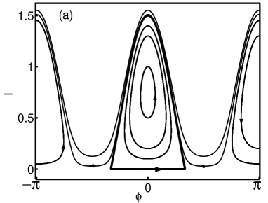
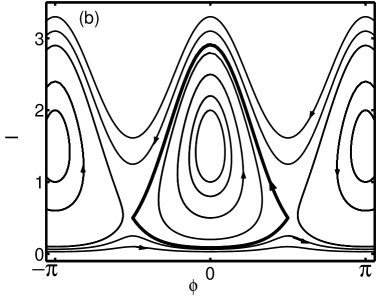
Figure 1: The phase portrait of the inviscid constant-frequency system (14) with detuning $\Delta=0.5$ (a) and $\Delta=2$ (b). Phase locking occurs inside the regions limited by the separatrix (denoted by the thick line). The saddle points are $[I^{*},\phi^{*}]=[0,\pm\arccos(-\Delta/2)]$ in case (a) and $[1/2,\pm\pi/2]$ in case (b). The phase portrait is periodic in $\phi$ with period $\pi$.

As the Hamilton’s function (15) is a constant of motion, the system is integrable. In particular, one can find the “nonlinear period”: the period of motion along a closed trajectory in the phase plane. Denoting the constant Hamilton’s function as $H_{0}$, we obtain

$$T_{nl}=2\int_{\phi_{-}}^{\phi_{+}}\frac{d\phi}{\left\{\left[\Delta+\cos(2\phi)\right]^{2}-4H_{0}\right\}^{1/2}}\,,$$ (16)

where $\phi_{\pm}=\pm\arccos(2\sqrt{H_{0}}-\Delta)/2$. For a zero detuning, and initial conditions very close to the fixed point $I_{*}=1/2$ and $\phi_{*}=0$ (so that $H_{0}\simeq\,1/4$), we obtain $T\simeq\pi$. This corresponds to small harmonic oscillations around the elliptic fixed point. In the physical units the period of small oscillations is $T_{nl}^{ph}\simeq\pi/(\varepsilon\omega_{1})$, that is much longer than the wave period.

II.2 Low-viscosity fluid

Taking into account a weak damping of the wave amounts to adding a linear damping term $2\gamma\dot{\eta}_{1}$ to the left side of Eq. (10), where $\gamma$ is defined in terms of the rate of loss of mechanical energy due to dissipation, Landau2 . The incorporation of only a linear damping term requires that $\gamma/\omega_{1}\ll\,1$, so that the damping is treated perturbatively. The specific damping mechanisms which contribute to the value of damping rate $\gamma$ are the bulk viscosity Landau2 , dissipation in the vicinity of the fixed walls Miles4 , dissipation at the free surface (especially if contaminated) Miles4 and contact line damping christiansen (see, e.g. Ref. christiansen for a review). In practice, one can interpret the damping rate as a phenomenological term, and determine it from a comparison with experiment.

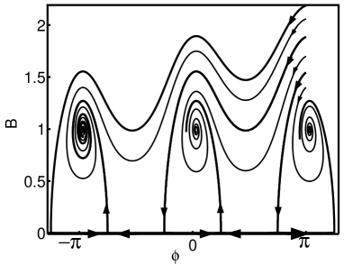
Figure 2: The phase portrait of the constant-frequency system (17) with a zero detuning and scaled damping rate $\Gamma=0.2$. The thick lines mark the separatrices, which pass through the saddle points $[B_{*},\phi_{*}]=[0,\pm\pi/4]$. The phase portrait is periodic in $\phi$ with period $\pi$.

Including the linear damping term in the first of Eqs. (13), we obtain:

$$\dot{B} = B\sin(2\phi)-\Gamma\,B\,,$$

$$\dot{\phi} = \cos(2\phi)-B^{2}+\Delta\,,$$ (17)

where $\Gamma=\gamma/(\varepsilon\omega_{1})>0$ is a dimensionless damping rate. It follows from the first of Eqs. (17), that non-trivial fixed points $B_{*}\neq 0$ can exist only when $\Gamma<1$, that is for a small enough viscosity. In this case, any trajectory on the phase plane of the system (except for trajectories with a zero measure) converges to a stable focus, see Fig. 2. This is in contrast to the inviscid case, where starting from initial conditions outside the separatrix leaves the trajectory phase-unlocked. The fixed points $[B_{*},\phi_{*}]$ of Eqs. (17) are determined by the values of $\Delta$ and $\Gamma$. Since Eqs. (17) [and Eqs. (13)] are invariant under the transformation $B\to-B$, one needs to consider only fixed points with positive amplitudes. Let $\sigma=\sqrt{1-\Gamma^{2}}$ and $\xi=\sqrt{1-\Delta^{2}}$. Let us also denote the critical damping rate

$$\Gamma_{cr}=\left[\frac{4}{5}-\frac{8\Delta}{25}\left(\Delta-\sqrt{\Delta^{2}+\frac{5}{4}}\right)\right]^{1/2}\,,$$ (18)

which will appear shortly. There are four different cases:

• $\Delta<-1$. No fixed points.

• $-1\leq\Delta<0$. For $\Gamma>\xi$, $[0,\arccos(-\Delta)/2]$ is a stable node, and $[0,-\arccos(-\Delta)/2]$ is a saddle point. For $0\,\leq\,\Gamma\,\leq\,\xi$, $[0,\pm\arccos(-\Delta)/2]$ are two saddle points, and $[(\sigma+\Delta)^{1/2},\arcsin(\Gamma)/2]$ is a stable fixed point. For $0\leq\Gamma<\Gamma_{cr}$ it is a stable focus, while for $\Gamma_{cr}<\Gamma\leq\xi$ it is a stable node.

• $0\leq\Delta<1$. For $\Gamma\geq\,1$, $[0,\arccos(-\Delta)/2]$ is a stable node, and $[0,-\arccos(-\Delta)/2]$ is a saddle point. For $\xi\,<\,\Gamma\,<\,1$, $[0,\arccos(-\Delta)/2]$ is a stable node, $[0,-\arccos(-\Delta)/2]$ and $[(\Delta-\sigma)^{1/2},\pi/2-\arcsin(\Gamma)/2]$ are two saddle points, and $[(\sigma+\Delta)^{1/2},\arcsin(\Gamma)/2]$ is a stable fixed point. For $\xi<\Gamma<\Gamma_{cr}$ it is a stable focus, while for $\Gamma_{cr}<\Gamma<1$ it is a stable node. For $0\,\leq\,\Gamma\,\leq\,\xi$, $[0,\pm\,\arccos(-\Delta)/2]$ are two saddle points, and $[(\sigma+\Delta)^{1/2},\arcsin(\Gamma)/2]$ is a stable focus.

• $\Delta\geq 1$. For $0\leq\Gamma\leq\,1$, $[(\sigma+\Delta)^{1/2},\arcsin(\Gamma)/2]$ is a stable fixed point. For $0\leq\Gamma<\Gamma_{cr}$ it is a stable focus, while for $\Gamma_{cr}<\Gamma\leq\,1$ it is a stable node, and $[(\Delta-\sigma)^{1/2},\pi/2-\arcsin(\Gamma)/2]$ is a saddle point.

Figure 3 shows two characteristic values of the scaled damping $\Gamma$ as functions of $\Delta$. The first one is $\Gamma_{cr}$ from Eq. (18). The second one is the maximum value of $\Gamma$ for which a nontrivial stable fixed point still exists. For $-1<\Delta<0$ this maximum value is equal to $\sqrt{1-\Delta^{2}}$, while for $\Delta\geq\,0$ it is equal to $1$. To conclude the brief review of the constant-frequency theory, we notice that the dependence of $B_{*}$ on $\Gamma$ exhibits a pitchfork bifurcation. Figure 4 shows the bifurcation diagram in case (c) for $\Delta=0.5$.

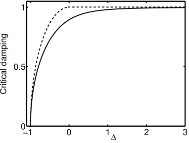
Figure 3: The solid line shows the critical scaled damping rate $\Gamma_{cr}$ as a function of the scaled detuning $\Delta$ [Eq. (18)]. For $\Gamma>\Gamma_{cr}$ (the over-damped case) a stable node is obtained, while for $\Gamma<\Gamma_{cr}$ a stable focus is obtained. The dashed line shows the maximum value of $\Gamma$ for which a nontrivial stable fixed point still exists. $\Gamma_{cr}$ is always below this maximum value.

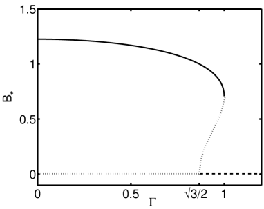
Figure 4: A combined bifurcation diagram of the constant-frequency system (17). Shown is the fixed-point amplitude $B_{*}$ versus $\Gamma$ for $\Delta=0.5$. The solid line shows the stable focus or stable node (depending on $\Gamma$), the dashed line shows the stable node and the saddle point [as described in case (c)], and the dotted lines show the unstable fixed points (saddle points and unstable focus). The bifurcation occurs at $\Gamma=\sqrt{1-\Delta^{2}}$, where the stable node $[B_{*},\phi_{*}]=[0,(1/2)\arccos(-\Delta)]$ becomes a saddle point. In the region $\sqrt{1-\Delta^{2}}<\Gamma<1$ both the stable focus, and the stable node exist.

III Chirped Faraday waves in an inviscid fluid

III.1 Governing equations, phase portrait, criteria and numerical examples

Now let the vibration frequency be time-dependent (chirped): $\omega=\omega(t)$. In general, the dimensionless parameter $\varepsilon=\omega^{2}a_{0}/g$ will also become time-dependent. For simplicity, we shall assume that $a_{0}$ also varies in time so that $\varepsilon=const$ constamp . Our objective is to keep a Faraday wave close to resonance in spite of its nonlinear frequency shift, so as to achieve a persistent growth of the wave amplitude. Like in other autoresonance schemes, the exact form of the function $\omega(t)$ is unimportant if this function satisfies three criteria:

1. The chirp sign coincides with the sign of the nonlinear frequency shift of the wave. For the standing Faraday waves $\omega(t)$ should decrease for the wave amplitude to increase.

2. The frequency chirp rate must be sufficiently small, so that the phase portrait of the system evolves adiabatically: $|\dot{\omega(t)}|\,T_{nl}\ll\omega(t)$, where $T_{nl}$ is the characteristic nonlinear period, see Eq. (16).

3. The dynamic frequency mismatch, which we define as the absolute value of the increment of the vibration frequency during one nonlinear period, $|\omega(t+T_{nl})-\omega(t)|$, should be small compared with the inverse nonlinear period, $T_{nl}^{-1}$. In physical units, this yields $\mu/(\varepsilon\omega_{1})^{2}\ll\,1$.

Criteria 1 and 2 have appeared in previous works on autoresonance Friedland1 , while criterion 3 is new. We shall see shortly that, in the problem of parametric autoresonance, criterion 3 is more restrictive than criterion 2.

The derivation of the equation of motion for the primary mode amplitude, for a slowly time-dependent driving frequency, goes along the same lines as in the case of a constant driving frequency. The resulting equation is (compare with Eq. (10)]:

$$\ddot{\eta}_{1}+\frac{1}{2}k_{1}^{2}(5\dot{\eta}_{1}^{2}\eta_{1}-3\omega_{1}^{2}\eta_{1}^{3})+\omega_{1}^{2}\left[1+4\varepsilon\cos(2\Phi(t))\right]\eta_{1}=0\,,$$ (19)

where $\Phi(t)=\int_{0}^{t}\omega(t^{\prime})\,dt^{\prime}$. If $\varepsilon$ is small, and the chirp rate is slow on the time scale of the wave period, one can again use, close to the parametric resonance, the method of averaging Khain . For concreteness, we assume in this work a constant chirp rate $\mu$:

$$\omega(t)=\omega_{1}-\mu\,t\,,$$ (20)

so that $\Phi(t)=\omega_{1}t-\mu t^{2}/2$. Introducing a scaled chirp rate $m=\mu/(\omega_{1}\varepsilon)^{2}$, and the same scaled time $\tau$ and amplitude $B$ as before [see Eq. (12)], we arrive at the following scaled equations:

$$\dot{B} = B\sin(2\phi)\,,$$

$$\dot{\phi} = \cos(2\phi)-B^{2}+m\tau,$$ (21)

where now $\phi(t)=\mu t^{2}/2+\phi_{1}(t)$, and the differentiation is done with respect to $\tau$. In the action-angle variables we obtain:

$$\dot{I} = 2I\sin(2\phi)\,,$$

$$\dot{\phi} = \cos(2\phi)-2I+m\tau\,.$$ (22)

Once $B(t)$ and $\phi(t)$ are found, one can immediately reconstruct the standing way profile $\eta(x,t)$ by using the Ansatz $\eta_{1}(t)=A_{1}(t)\cos\left[\omega_{1}t+\phi_{1}(t)\right]$ and the “enslaving relation” (8) in the second of equations (II.1). Therefore, in the rest of the paper we shall focus on Eqs. (22) which coincide, up to notation, with those obtained by Khain and Meerson Khain , who investigated parametric autoresonance in a nonlinear oscillator. Equations similar to (22) also appear in the problem of the second-harmonic autoresonance in an externally driven oscillator Lazar7 .

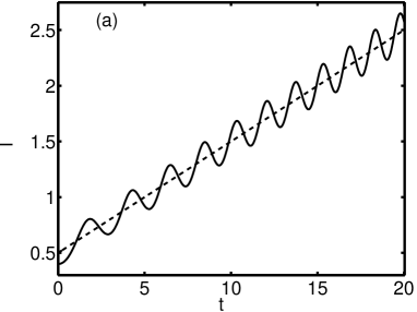
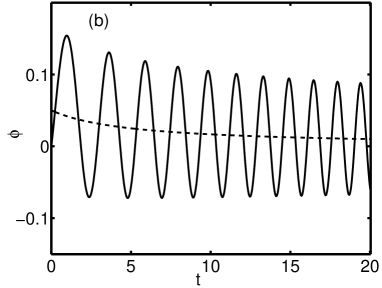
Figure 5: Parametric autoresonance in an inviscid fluid. Shown are the action $I$ (a) and the phase $\phi$ (b) as functions of time. The parameters are $m=0.2$, $I(0)=0.4$, $\phi(0)=0$, and a zero initial detuning. The solid lines shows numerical solutions. The dashed lines show the trends $I_{*}(t)$, given by Eq. (24) (a) and $\phi_{*}(t)$, given by Eq. (25) (b).

The Hamilton’s function of the system (22) is time dependent:

$$H(I,\phi)=I\cos(2\phi)-I^{2}+m\tau I\,,$$ (23)

so $H$ is not a constant of motion anymore. In the following we shall use $t$ for the slow time $\tau$.

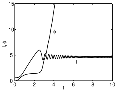
Figure 6: Breakdown of parametric autoresonance in an inviscid fluid in the case of $m=5.5>m_{cr}$. The parameters are $m=5.5$, $I(0)=0.6$, $\phi(0)=0$, and a zero initial detuning. Shown are the action $I(t)$ and the phase $\phi(t)$ found numerically.

Figure 5 shows an example of parametric autoresonance: a persistent phase locking and a systematic growth of $I$ with time, with some oscillations on top of the systematic growth. Here the scaled chirp rate $m$ is less than some critical value $m_{cr}$ for these initial conditions. Figure 6 illustrates breakdown of autoresonance, observed when $m>m_{cr}$. As in other instances of autoresonance, a theory of parametric autoresonance appeals to the constant-frequency theory. Comparing Eqs. (22) and (14), one can see that the term $mt$ plays the role of an effective (time-dependent) detuning. Therefore, when the chirp rate is small, $m\ll\,1$, the phase portrait of the system almost coincides with that of the autonomous equations (14) (see Fig. 1), except that now it changes with time according to the current value of the effective detuning. The change of the phase portrait is adiabatically slow, except at times $t\simeq-1/m$ and $1/m$ (corresponding to $\Delta=-1$ and $1$, respectively), when bifurcations occur. One consequence of the adiabatic evolution is that Eqs. (22) have “quasi-fixed” points. The most important stable quasi-fixed point $[I_{*}(t),\phi_{*}(t)]$ can be found by assuming that $\phi_{*}(t)\ll 1$, and that it varies with time slowly. Then the second of Eqs. (22) yields, in the leading order,

$$I_{*}\simeq\frac{1}{2}\left(1+mt\right)\,.$$ (24)

Substituting this into the first of Eqs. (22), we obtain

$$\phi_{*}\simeq\frac{m}{4(1+mt)}\,.$$ (25)

The stable quasi-fixed point, or trends (24) and (25), previously found by Khain and Meerson Khain (see also Ref. Lazar7 ), are the essence of parametric autoresonance. Shown in Fig. 5 are $I(t)$ and $\phi(t)$ found numerically, and the trends (24) and (25). The trend (24) corresponds to a steady growth of the wave amplitude: $B_{*}(t)=[2I_{*}(t)]^{1/2}\simeq(mt+1)^{1/2}$. The important phase trend (25) was overlooked in Ref. Lazar7 . Notice that, at scaled time $t\gg 1$, the phase trend $\phi_{*}\simeq 1/(4t)$ becomes independent of the chirp rate $m$. Importantly, for the expressions (24) and (25) to be valid, one can either demand $m\ll 1$, or go to long times: $t\gg 1$. Therefore, the stable quasi-fixed point keeps its meaning, at long times, even at finite (non-small) $m$.

We found that, surprisingly, unstable quasi-fixed points of the chirped system also play an important role in the dynamics. The unstable points are analogs of the constant-frequency saddle points discussed in the previous section [see the text following Eq. (15)]. To find the locations of the unstable quasi-fixed points in the leading order, one can simply replace the detuning $\Delta$ by $mt$. Therefore, on the time interval $0<t<1/m$, there are two saddle quasi-fixed points $[I_{*},\phi_{*}]\simeq\,[0,\pm(1/2)\arccos(-mt)]$. These points disappear at $t\simeq 1/m$, and a new saddle points appears: $[I_{*},\phi_{*}]\simeq\,[(mt-1)/2,\pi/2)]$. These expressions (including the boundaries of the corresponding time intervals) are valid in the leading order in $m\ll 1$. Higher-order corrections can be also calculated.

Now we are in a position to discuss criteria 2 and 3 for parametric autoresonance in this system. For a constant chirp rate $\mu$ [see Eq. (20)], criterion 2 can be written, in the physical units, as $\mu(\varepsilon\omega)^{-1}<\omega$, or $\mu<\varepsilon\omega^{2}$. Now, the dynamic frequency mismatch, acquired by the chirped system during time $T_{nl}$, can be estimated as $\mu T_{nl}\sim\mu/(\varepsilon\omega)$. Criterion 3 demands that this quantity be small compared to $T_{nl}^{-1}\sim\varepsilon\omega$, which yields $\mu<\varepsilon^{2}\omega^{2}$. As $\varepsilon$ is small, criterion 3 is more restrictive than criterion 2. In the scaled variables, criterion 3 has the form of $m<1$, as can be expected from the form of scaled Eqs. (22). The inequalities here are written up to numerical factors which depend on the initial conditions, see below.

One more convenient description of the chirped system can be achieved if we rewrite Eqs. (22) as a second order equation for the phase:

$$\ddot{\phi}+2mt\sin(2\phi)+\sin(4\phi)-m=0\,,$$ (26)

or

$$\ddot{\phi}+\frac{\partial\,V(\phi,t)}{\partial\phi}=0\,,$$ (27)

where we have introduced a time-dependent potential

$$V(\phi,t)=-\frac{1}{4}\cos(4\phi)-mt\cos(2\phi)-m\phi\,.$$ (28)

This suggests new canonical variables $\phi$ and $u=\cos(2\phi)-2I+mt$, so that in the new time-dependent Hamiltonian, $H(\phi,u,t)=u^{2}/2+V(\phi,t)$, there is a clear separation between the potential energy and the kinetic energy. The new Hamiltonian describes a “particle” of a unit mass and velocity $u=\dot{\phi}$, moving in a time-dependent potential $V$. This picture is useful for a qualitative analysis of the dynamics of the “particle” when $m$ is small, so the potential slowly varies in time, see Fig. 7. In the variables $u,\phi$ the stable quasi-fixed point becomes (approximately) $[0,(m/4)(1+mt)^{-1}]$, while the saddle points are $[0,\pm(1/2)\arccos(-mt)]$ at $0<t<1/m$, and $[0,\simeq\pm\,\pi/2]$ at $t>1/m$. We shall see shortly that each of the unstable points $[0,(1/2)\arccos(-mt)]$ and $[0,\simeq\pi/2]$ plays an important role in this system.

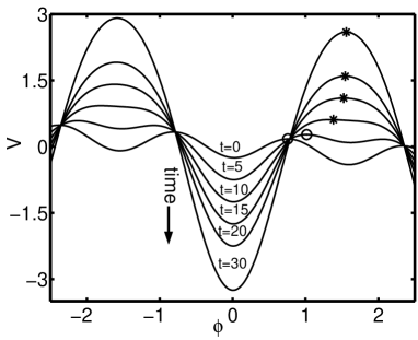
Figure 7: The time-dependent potential $V(\phi,t)$, Eq. (28), is shown as a function of $\phi$ for several consecutive times starting from $t=0$. The scaled chirped rate $m=0.1$. The potential well at $\phi\simeq\phi_{*}(t)$ deepens with time starting from $t=0$. At $0<t<1/m$ there is a potential barrier at $\phi\simeq(1/2)\arccos(-mt)$ (denoted by the circle), which disappears at $t\simeq 1/m$. At $t\simeq 1/m$ a new potential barrier appears close to $\phi=\pi/2$ and heightens with time (denoted by the asterisk).

Let us consider two typical cases of parametric autoresonant excitation of a Faraday wave. In the first case one first excites the wave at a constant frequency, so that the initial values of the action and phase are in the vicinity of the stable fixed point. Then, upon slowly reducing the driving frequency, one keeps the phase locked, as our “particle” oscillates in a potential well which slowly deepens with time, see Fig. 7. In the second case one starts the autoresonant driving from an almost zero wave amplitude. Here the saddle point $[I_{*},\phi_{*}]\simeq\,[0,(1/2)\arccos(-mt)]$ plays an important role. Indeed, the stable manifold of this quasi-fixed point is along the $\phi$ axis. Therefore, no matter what the initial phase is, the phase approaches, on a time scale ${\cal O}(1)$, the saddle point. The unstable manifold of this saddle point is along the $I$ axis, so $I(t)$ will grow with time. Still, if $I(t=0)$ is small enough, $I(t)$ remains small during this time scale ${\cal O}(1)$. Therefore, phase locking is always achieved at this stage, so the time interval $0<t<1/m$ can be called the “trapping stage”. Later on $I(t)$ grows significantly but, as we found numerically, the “particles” remain inside the (slowly expanding) separatrix $I=\cos(2\phi)+mt$. As a result, the phase starts to perform large-amplitude oscillation around the stable quasi-fixed point, and phase locking persists.

One more alternative description of the system of equations (21) is in terms of the complex amplitude $\psi(t)=B(t)\exp[i\phi(t)]$:

$$i\psi_{t}+\psi^{*}-(|\psi|^{2}-mt)\psi=0\,,$$ (29)

where the subscript $t$ denotes differentiation with respect to the slow time. The long-time behavior of $I_{*}$ can be obtained by looking at the asymptotic solutions of Eq. (29) at $t\rightarrow\infty$. For a solution such that $|\psi|$ grows with time like a power law, the leading terms are those in the parentheses. This immediately yields

$$|\psi(t)|\simeq(mt)^{1/2}\,,$$ (30)

which corresponds to the leading term (when $mt\gg\,1$) of Eq. (24), and describes a phase-locked wave [here $\phi$ stays close to zero, see Eq. (25)]. On the contrary, if $|\psi(t)|$ remains bounded and small, the first term of Eq. (29) is balanced by the last one, and we obtain

$$\psi(t)=\psi_{0}\exp\left(imt^{2}/2\right)\,,$$ (31)

where $\psi_{0}\equiv|\psi_{0}|\exp(i\phi_{0})=const.$ This solution corresponds to an unlocked phase $\phi(t)=\phi_{0}+mt^{2}/2$ and a constant amplitude $|\psi_{0}|$. Of course, the phase of the wave $\phi_{1}(t)=\phi(t)-mt^{2}/2$, which is defined by the Ansatz $\eta_{1}(t)=A_{1}(t)\cos\left[\omega_{1}t+\phi_{1}(t)\right]$ (where $t$ is the physical time), stays constant in this regime, and is equal to $\phi_{0}$.

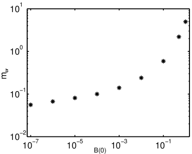
Figure 8: The critical chirp rate $m_{cr}$ as a function of the initial amplitude $B(0)$ for $\phi(0)=0$.

We determined numerically, for several typical classes of initial conditions, the critical value of $m$, $m=m_{cr}$, which separates the phase locking regime from the phase unlocking regime alternative . At a fixed initial phase $\phi(t=0)=0$, $m_{cr}$ grows with the initial amplitude $B(t=0)$, at least until the scaled amplitude becomes of order unity, see Fig. 8. This result agrees with those obtained by Fajans et. al. (see Fig. 3 in Ref. Lazar7 ) who presented them in terms of $\varepsilon_{cr}$ versus $\mu$. When starting from the stable quasi-fixed point: $I(t=0)=1/2$ and $\phi(t=0)=0$, we found that $m_{cr}\simeq\,4.963$.

We also found $m_{cr}$ as a function of the initial phase, for a given, and very small, initial amplitude, see Fig. 9. This dependence is relatively weak. The largest $m_{cr}$ is obtained for $\phi=\pi/4$, the smallest one for $\phi=-\pi/4$.

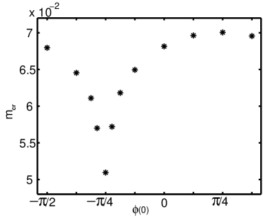
Figure 9: The critical chirp rate $m_{cr}$ as a function of the initial phase $\phi(0)$, for a very small initial amplitude $B(0)=10^{-6}$.

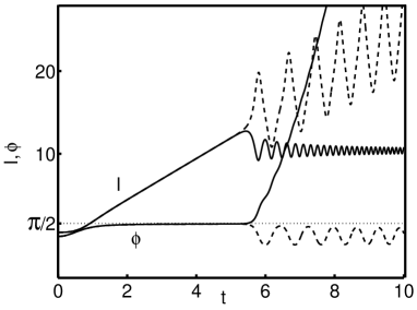
Figure 10: Autoresonance and its breakdown for $m$ very close to $m_{cr}\simeq 4.963$. The initial conditions are $\phi(t=0)=0$ and $I(t=0)=1/2$. The dashed lines show the phase-locked solutions for the phase and action for $m$ just below $m_{cr}$, while the solid lines show the phase-unlocked solutions for $m$ just above $m_{cr}$.

What is the signature of the special case $m=m_{cr}$? At $m<m_{cr}$ the phase oscillates in time. As $m$ approaches $m_{cr}$ from below, the onset of the phase oscillations is delayed more and more, see Fig. 10. Now, at $m>m_{cr}$ the phase initially changes slowly and then rapidly escapes to infinity. As $m$ approaches $m_{cr}$ from above, the point of rapid departure of the phase is delayed more and more, as shown in Fig. 10. This suggests that, in the special case $m=m_{cr}$ the phase neither oscillates around a trend, nor departs from it. Instead, the phase monotonically approaches $\pi/2$. Looking at the effective potential, shown in Fig. 7, one realizes that, in the special case $m=m_{cr}$, our “particle” neither oscillates in the potential well (which would correspond to phase locking), nor escapes from the well (which would correspond to phase unlocking). Instead, the “particle” lands, at $t=\infty$, on the peak of the potential at $\phi=\pi/2$. In the following we shall find the asymptotic form of this special trajectory.

III.2 Perturbative solutions

In this subsection we present three perturbative analytic solutions which illustrate the basic features of parametric autoresonance: persistent resonant growth, capture into resonance and the limiting trajectory which separates between phase locking and unlocking. In each of the three cases, a local analysis around one of the quasi-fixed points of the system is required.

III.2.1 In the vicinity of the stable quasi-fixed point

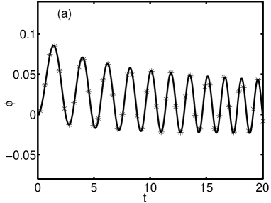
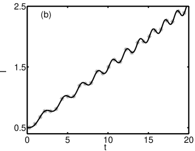
Figure 11: The phase $\phi(t)$ (a) and the action $I(t)$ (b) as functions of time for $m=0.2$, $\phi(0)=0$ and $I(0)=1/2$. The asterisks mark the asymptotic solutions given by Eqs. (36) (a) and (37) (b). The solid lines mark the numerical solutions.

Let us linearize Eq. (26) in the vicinity of $\phi=0$. As discussed above, this requires either a small chirp rate, $m\ll 1$, or a long time, $t\gg 1$. We obtain:

$$\ddot{\phi}+4(1+mt)\phi=m\,.$$ (32)

We look for the solution in the form

$$\phi(t)=\frac{m}{4(1+mt)}+\delta\phi(t)\,,$$ (33)

where the first term is the phase trend (25). Neglecting higher-order terms, we arrive at the Airy equation

$$\ddot{\delta\phi}+4(1+mt)\delta\phi=0\,,$$ (34)

whose general solution is Abramowitz :

$$\delta\phi(\tau) = C_{1}\,Ai\left[-\left(\frac{2}{m}\right)^{2/3}(1+mt)\right]+$$ (35)

$$C_{2}\,Bi\left[-\left(\frac{2}{m}\right)^{2/3}(1+mt)\right]\,.$$

Here $Ai(\tau)$ and $Bi(\tau)$ are the Airy functions of the first and second kind, and $C_{1}$ and $C_{2}$ are constants depending on the initial conditions. Using the large-argument expansion of $Ai(-z)$ and $Bi(-z)$ Abramowitz , we obtain:

$$\phi(t)\simeq\frac{m}{4(1+mt)}+\frac{A}{(1+mt)^{1/4}}\sin\!\left[\frac{4(1\!+\!mt)^{3/2}}{3m}+\xi\right]\,,$$ (36)

where $A$ and $\xi$ are new constants. The action $I(t)$ can be found using the second of Eqs. (22):

$$I(t)\simeq\frac{mt+1}{2}-A(1+mt)^{1/4}\cos\!\left[\frac{4(1\!+\!mt)^{3/2}}{3m}+\xi\right]\,.$$ (37)

The first terms in Eqs. (36) and (37) are the systematic trends (25) and (24). The solutions (36) and (37) coincide, up to notation, with the WKB-solutions obtained in Ref. Khain . Fig. 11 shows excellent agreement between the analytical solutions (36) and (37) and numerical solutions.

III.2.2 Capture into resonance

Now we consider the case of driving a Faraday wave starting from a very small amplitude and a large initial detuning, that is far from resonance. Here one is interested in the capture into resonance. In the case of external autoresonance this phenomenon has been extensively studied by Friedland Friedland1 . In the case of parametric autoresonance this phenomenon has not been addressed, although equations similar to (22) were analyzed in Ref. Lazar7 in the context of the second-harmonic autoresonance in an externally driven oscillator.

We start, in Eqs. (21), at a large negative time $t_{0}<0$, and assume that the initial detuning $mt_{0}$ is very large in the absolute value, while the initial scaled amplitude $B(t=t_{0})$ is much less than unity. As long as $B(t)\ll 1$, one can neglect the $B^{2}$-term in the second of Eqs. (21):

$$\dot{\phi}=\cos(2\phi)+mt\,.$$ (38)

This equation describes two distinct stages of the dynamics. In the first stage $t$ is large and negative, and $|mt|\gg 1$. Therefore, the term $mt$ is dominant, so Lazar7

$$\phi\simeq\phi(t_{0})+\frac{m}{2}(t-t_{0})^{2}\,.$$ (39)

During this pre-locking stage, the phase varies rapidly. The second stage occurs roughly at $-1/m<t<1/m$. Here the two terms on the right hand side of Eq. (38) are comparable. As $m\ll 1$, the duration of this stage is long compared with unity, and the phase approaches, on a time scale ${\cal O}(1)$, the unstable quasi-fixed point

$$\phi_{*}(t)\simeq\frac{\arccos(-mt)}{2}-\frac{m}{4[1-(mt)^{2}]^{1/2}}\,,$$ (40)

where we have included the next-order correction in $m$. As noted previously, this quasi-fixed saddle point ceases to exist at $t>1/m$; the correction term in Eq. (40) is invalid too close to $t=1/m$. We call this regime “linear phase locking” stage.

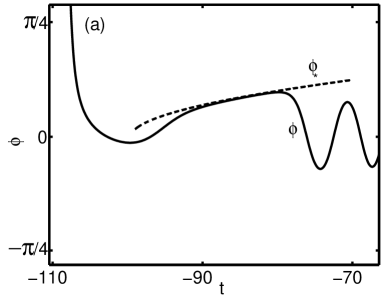
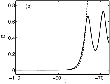
Figure 12: The dynamics of the system in the linear phase locking stage $-1/m<t<1/m$. The phase $\phi(t)$ (a) and amplitude $B(t)$ (b), found numerically, are shown by solid lines. The quasi-fixed saddle point $\phi_{*}(t)$ [Eq. (40)] (a) and the amplitude [Eq. (43)] (b) are denoted by dashed lines. The initial conditions are $t_{0}=-400$, $\phi(t_{0})=0$, and $B(t_{0})=10^{-6}$, the scaled chirp rate $m=0.01$. It can be seen that, as $B$ becomes comparable to $1$, the linear theory breaks down.

Let us obtain the dependence of $B$ on time in the pre-locking and linear phase locking stages. In the pre-locking stage $\phi(t)$ is given by Eq. (39). Then the first of Eqs. (21) yields

$$B(t)\simeq B(t_{0})\exp\left\{\int_{t_{0}}^{t}\sin\left[m(s-t_{0})^{2}+2\phi(t_{0})\right]ds\right\}$$ (41)

(the integral can be expressed through the Fresnel integral). At this stage $B(t)$ oscillates rapidly, because of the rapid and monotonic change of the phase. At the linear phase locking stage, $\phi(t)\simeq\phi_{*}(t)$ as given by Eq. (40). Then, neglecting higher-order terms in $m$, we arrive at the equation

$$\dot{B}\simeq B\sqrt{1-(mt)^{2}}$$ (42)

which yields

$$B\simeq B_{2}\exp\left\{\frac{1}{2}\left[t\sqrt{1-(mt)^{2}}+\frac{\arcsin(mt)}{m}\right]\right\}\,,$$ (43)

where $B_{2}$ is a constant determined by the initial conditions.

Equation (43) breaks down when the earliest of the two events occurs: $t$ becomes larger than $1/m$, or $B(t)$ becomes comparable to unity, so that one cannot neglect the $B^{2}$-term in the second of Eqs. (21). The phase starts to oscillate, while the amplitude both oscillates and grows, see Fig. 12, and the system enters the autoresonance regime.

Similar results are observed when starting from a small amplitude and a zero initial detuning (that is, in exact linear resonance). Therefore, when the initial amplitude is very small, and $m\ll\,1$, phase locking is very robust.

III.2.3 Critical chirp rate and the limiting trajectory

As we have seen numerically, when $m$ approaches the critical value $m_{cr}$, the phase $\phi$ approaches $\pi/2$ at $t\gg 1$. Let us assume that, at a time $t_{0}$, $\phi$ is already in the vicinity of $\pi/2$: $\phi=\pi/2-\delta\phi$, where $\delta\phi\ll 1$. Linearizing Eq. (26), we obtain

$$\ddot{\delta\phi}-4\delta\phi(mt-1)=-m\,.$$ (44)

To find the trend, we neglect the term $\ddot{\delta\!\phi}$. Therefore, at $t\gg 1$, we obtain $\delta\phi\simeq 1/(4t)$, so

$$\phi_{*}(t)\simeq\frac{\pi}{2}-\frac{1}{4t}\,.$$ (45)

Using the second of Eqs. (22), we obtain the respective trend of $I(t)$:

$$I_{*}(t)\simeq\frac{mt}{2}-\frac{1}{2}\,.$$ (46)

At this stage we notice that Eqs. (45) and (46) describe, at $t\gg 1$, one of the unstable (saddle) quasi-fixed points of the system: the one that appears close to $t=1/m$. This again shows that adiabaticity holds not only at $m\ll 1$, but also at $t\gg 1$.

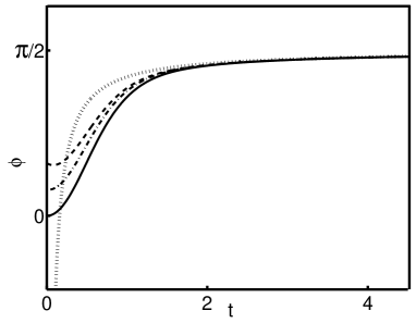
Figure 13: Numerical solutions for the phase $\phi(t)$, for three different initial conditions, versus the universal asymptotics (45), denoted by the dotted line. The solid, dashed-dotted and dashed lines show the phase dynamics when starting from $\phi(0)=0$ (here $m\simeq m_{cr}\simeq\,4.963$), $1/4$ (here $m\simeq m_{cr}\simeq\,6.237$), and $1/2$ (here $m\simeq m_{cr}\simeq\,7.094$), respectively. $I(0)=1/2$ in all three cases.

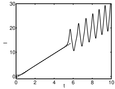
Figure 14: Shown is $I(t)$ for $m$ just below $m_{cr}\simeq 4.963$. The solid line shows the numerical solution, starting from $I(0)=1/2$ and $\phi(0)=0$. The dashed line shows the trend (46).

Now consider small deviations from the unstable trends (45) and (46). Putting $\phi=\pi/2-1/(4t)-\delta\phi(t)$, we again arrive at the Airy equation for $\delta\phi(t)$. Its general solution is $\delta\phi(t)=C_{1}Ai[(4m)^{1/3}t]+C_{2}Bi[(4m)^{1/3}t]$, where $C_{1}$ and $C_{2}$ are determined by the initial conditions. Assuming $m^{1/3}t\gg 1$, we employ the asymptotics of the Airy functions Abramowitz :

$$Ai(z)\simeq\frac{\exp\left[-(2/3)z^{3/2}\right]}{2\sqrt{\pi}z^{1/4}}\,,\;\;Bi(z)\simeq\frac{\exp\left[(2/3)z^{3/2}\right]}{\sqrt{\pi}z^{1/4}}$$ (47)

at $z\gg\,1$. The exponentially decaying term is negligible. The exponentially growing term describes instability of the special trajectory with respect to small perturbations. This instability occurs both at $m<m_{cr}$ (when the phase leaves the vicinities of the saddle point and goes to the vicinity of the stable quasi-fixed point), and at $m>m_{cr}$ (when the phase locking terminates). For the special trajectory, obtained for $m=m_{cr}$, the coefficient $C_{2}$ must vanish, which brings us back to Eqs. (45) and (46), where we must put $m=m_{cr}$. Now it is clear that the asymptotic behavior of the $\phi_{*}(t)$ at $m=m_{cr}$ is independent of $m_{cr}$ and, therefore, on the initial conditions. On the contrary, the asymptotic behavior of $I_{*}(t)$ at $m=m_{cr}$ does depend on $m_{cr}$ and, therefore, on the initial conditions. Unfortunately, the local analysis does not enable one to find the value of $m_{cr}$ analytically.

Figures 13 and 14 show the behavior of the system when $m$ is very close to (just below) $m_{cr}$. Figure 13 shows that, after a time ${\cal O}(1)$, the phase follows the trend (45), independently of the initial conditions (and of the value of $m_{cr}$). Figure 14 shows that, after a time of ${\cal O}(1)$, good agreement between $I(t)$, found numerically, and the trend (46) holds until the time when the “particle” leaves the vicinity of the unstable point and transfers to the vicinity of the stable point.

IV Chirped Faraday waves in a low-viscosity fluid

We now account for a small viscosity and briefly describe the dynamics of the phase and amplitude of the primary mode in the case of a slowly time-dependent vibration frequency. The weakly nonlinear governing equations are obtained by analogy with Eqs. (17):

$$\dot{B} = B\sin(2\phi)-\Gamma\,B\,,$$

$$\dot{\phi} = \cos(2\phi)-B^{2}+mt\,,$$ (48)

where $t$ is the slow time as before. For $\Gamma<1$, there exists a stable quasi-fixed point which describes autoresonant excitation of the wave:

$$B_{*} \simeq \left[(1-\Gamma^{2})^{1/2}+mt\right]^{1/2}\,,$$

$$\phi_{*} \simeq \frac{1}{2}\arcsin(\Gamma)+\frac{m}{4[1-\Gamma^{2}+mt(1-\Gamma^{2})^{1/2}]}\,.$$ (49)

When $\Gamma\ll 1$, Eqs. (49) become

$$B_{*}\simeq\sqrt{1+mt}\,,\;\;\;\phi_{*}\simeq\frac{\Gamma}{2}+\frac{m}{4(1+mt)}\,.$$ (50)

Figure 15 shows a projection on the $(\phi,B)$ plane of a three-dimensional trajectory in the space of $\phi$, $B$ and $t$. One can see phase locking and a steady growth of the wave amplitude with time.

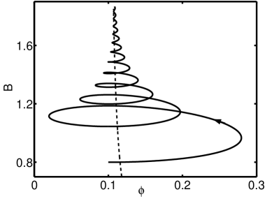
Figure 15: Parametric autoresonance in the presence of viscosity. Shown is a projection of a three-dimensional trajectory in the space of $\phi$, $B$ and $t$, upon the $(\phi,B)$-plane. The solid line shows a numerical solution, the dashed line shows the trends (48). After several nonlinear cycles, the trajectory converges into a (slowly time-dependent) stable focus, which moves upwards. The parameters are $\Gamma=0.2$, $m=0.1$, $B(0)=0.8$, $\phi(0)=0.1$, and a zero initial detuning.

Figures 16 and 17 show two different regimes of autoresonant growth in the dissipative system. Shown in the two figures are the primary mode amplitude versus time for the scaled damping rates $\Gamma<\Gamma_{cr}$ and $\Gamma>\Gamma_{cr}$, respectively. As the initial detuning is zero, $\Gamma_{cr}=2/\sqrt{5}=0.89\dots$ here, see Eq. (18). Figure 16 shows decaying oscillations on top of the amplitude growth, given by the first of Eqs. (49). Figure 17 shows a non-oscillatory regime of the amplitude growth. Figure 18 shows breakdown of autoresonance when the chirp rate $m$ exceeds a critical value.

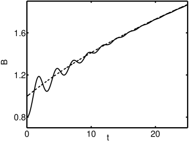
Figure 16: Parametric autoresonance in the presence of viscosity. Shown is the amplitude $B(t)$ versus time for a subcritical damping. The solid line denotes a numerical solution, while the dashed line shows the trend $B_{*}(t)$, see Eq. (49). The parameters are the same as in Fig. 15.

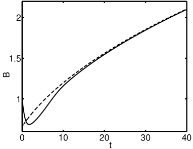
Figure 17: Parametric autoresonance in the presence of viscosity. Shown is the amplitude $B(t)$ versus time for a supercritical damping. The solid line denotes the amplitude $B(t)$ found numerically, and the dashed line denotes its trend $B_{*}(t)$, see Eq. (49). The parameters are $\Gamma=0.9$, $m=0.1$, $B(0)=1$, $\phi(0)=0.25$, and a zero initial detuning.

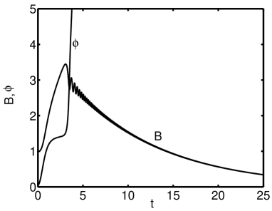
Figure 18: Breakdown of autoresonance in the presence of viscosity. Shown are the amplitude $B(t)$ and the phase $\phi(t)$, for $m\simeq\,4.4$ (just above $m_{cr}$) for the initial conditions $B(0)=1$ and $\phi(0)=0.05$, and for $\Gamma=0.1$. One can see that, after a strong transient excitation, the phase unlocks, and the amplitude decays.

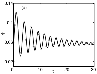
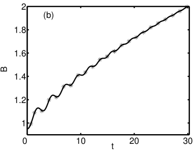
Figure 19: The phase $\phi(t)$ (a) and the amplitude $B(t)$ (b) as functions of time in the presence of small viscosity. The parameters are $m=0.1$, $\Gamma=0.1$. The initial conditions are $\phi(0)=0.05$ and $B(0)=0.95$. The asterisks mark the analytical solutions, the solid lines show numerical solutions.

Similarly to the inviscid case, one can rewrite the governing equations (48) as a single equation for the complex amplitude, $\psi=B\exp(i\phi)$:

$$i\psi_{t}+\psi^{*}-(|\psi|^{2}-mt-i\Gamma)\psi=0\,.$$ (51)

Assuming a solution growing in time (that is, phase locked solution), we obtain, at $t\gg 1$, $B=|\psi|\simeq(mt)^{1/2}$, as before.

Equations (48) can be also rewritten as a single second-order equation for $\phi(t)$:

$$\ddot{\phi}+2\Gamma\dot{\phi} + \sin(4\phi)+2mt\sin(2\phi)$$ (52)

$$- 2\Gamma\cos(2\phi)=2\Gamma mt+m$$

[compare it with Eq. (26)]. This equation is convenient for a perturbative treatment in the vicinity of the stable quasi-fixed point. For $\Gamma\ll 1$, we can linearize Eq. (52) around $\phi=0$:

$$\ddot{\phi}+2\Gamma\dot{\phi}+4(1+mt)\phi=2\Gamma\!(1+mt)+m\,.$$ (53)

Now we substitute $\phi(t)=\phi_{*}(t)+\delta\phi(t)$, where $\phi_{*}$ is given by the second of Eqs. (50), and obtain a linear equation

$$\ddot{\delta\phi}+2\Gamma\dot{\delta\phi}+4(1+mt)\phi=0\,.$$ (54)

Its approximate solution, at $m\ll 1$ and $\Gamma\ll 1$, can be written as

$$\delta\phi\simeq\frac{A\,e^{-\Gamma t}}{(1+mt)^{1/4}}\sin\left[\frac{4(1+mt)^{3/2}}{3m}+\xi\right]\,,$$ (55)

where $A$ and $\xi$ are constants depending on the initial conditions. The respective solution for $B(t)$ is

$$B\simeq(1+mt)^{1/2}-\frac{A\,e^{-\Gamma t}}{(1+mt)^{1/4}}\cos\left[\frac{4(1+mt)^{3/2}}{3m}+\xi\right]\,,$$ (56)

These solutions are simple extensions of the non-viscous perturbative solutions. A comparison with numerical solutions is shown in Fig. 19, and excellent agreement is observed.

In the viscous case the critical value $m_{cr}$ of the scaled chirp rate $m=\mu/(\varepsilon\omega_{1})^{2}$ depends on the scaled damping rate of the wave $\Gamma=\gamma/(\varepsilon\omega_{1})$. Figure 20 shows this dependence, which we found numerically when starting at $t=0$ from the stable fixed point of Eqs. (17) with $\Delta=0$, that is from $B_{*}=(1-\Gamma^{2})^{1/4}$ and $\phi_{*}=(1/2)\arcsin(\Gamma)$. One can see that, as $\Gamma$ increases, the critical chirp rate goes down monotonically. As $\Gamma$ approaches $1$, $m_{cr}$ goes to $0$. Notice that, once we return to the physical (dimensional) critical chirp rate $\mu_{cr}$ and the wave damping rate $\gamma$, the dependence of $\mu_{cr}$ on $\varepsilon$, at fixed $\gamma$, is not a power law.

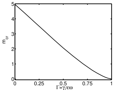
Figure 20: The critical scaled chirp rate $m_{cr}=\mu_{cr}/(\varepsilon^{2}\omega_{1}^{2})$ versus the scaled damping rate of the wave $\Gamma=\gamma/(\varepsilon\omega_{1})$, as described by Eqs. (48). The initial amplitude and phase correspond to the stable fixed point of Eqs. (17) with $\Delta=0$.

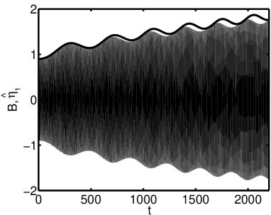
Figure 21: $B(t)$ (the thick solid line) and $\hat{\eta}_{1}$ (the thin solid line) versus time. The parameters are $\Gamma=0.006$, $m=0.18$, $\varepsilon=0.006$, $\hat{\eta}_{1}(0)=B(0)=0.9$ and $\dot{\hat{\eta}}_{1}(0)=\phi(0)=0$.

Finally, we tested the accuracy of our reduced equations (48). We compared numerical solutions of Eqs. (48) with numerical solutions of the unreduced equation of motion (19) for the primary mode amplitude $\eta_{1}(t)$, with a linear damping term added. Rescaling the time $\tau=\omega_{1}t$, and the amplitude $\hat{\eta}_{1}=(k_{1}\eta_{1})/(2\sqrt{\varepsilon})$, one can rewrite the unreduced equation as

$$\ddot{\hat{\eta}}_{1} + 2\varepsilon\Gamma\dot{\hat{\eta}}_{1}+10\varepsilon\dot{\hat{\eta}}_{1}^{2}\hat{\eta}_{1}-6\varepsilon\hat{\eta}_{1}^{3}+$$ (57)

$$+ \hat{\eta}_{1}\left[1+4\varepsilon\cos\left(2\tau-m\varepsilon^{2}\tau^{2}\right)\right]=0\,.$$

A typical example of this comparison is shown in Fig. 21, and a fairly good agreement between the envelope of $\hat{\eta}_{1}(t)$ and the amplitude $B(t)$ is observed.

V Discussion

This paper presents a theory of weakly nonlinear standing gravity waves, parametrically excited by weak vertical vibrations with a down-chirped vibration frequency. We have shown that autoresonance phase locking and a steadily growing wave amplitude can be achieved despite the nonlinear frequency shift of the wave. For typical initial conditions we have found the critical chirp rate, above which autoresonance breaks down. When starting from a very small wave amplitude, and slowly passing through resonance, phase locking always occurs. We have obtained approximate analytical expressions for the time-dependent wave profile in different regimes. We have demonstrated that each of the three quasi-fixed points of the reduced dynamic equation, describing the primary mode, plays an important role in the dynamics of the system and/or in determining the critical chirp rate.

Parametric autoresonance in Faraday waves is a robust phenomenon, and its experimental observation should not be difficult. To test our theory, one should use a quasi-two-dimensional tank with a low-viscosity liquid, and perform measurements of the standing wave elevation as a function of time. The long-term wave amplitude trend [see the first of Eqs. (49)], and the critical chirp rate (see Fig. 20), give examples of quantitative predictions of the theory that can be tested in experiment. One such experiment is presently under way Oded .

The applicability of the weakly nonlinear theory presented in this work is limited to weak forcing and weak damping. Our analysis neglected higher order terms in $\varepsilon$, which include a nonlinear forcing Miles3 , a cubic damping Miles3 ; douady ; milner , a small correction to the linear detuning/frequency shift, a quintic conservative term decent , etc. These terms can be included in the theory of autoresonance in order to achieve a better accuracy. Importantly, once these higher-order terms are added to the constant-frequency model [Eq. (17)], the non-trivial stable fixed point will exist only up to a certain value of the frequency detuning Miles3 ; douady ; milner ; decent . Therefore, in experiment, the autoresonant growth of the wave is expected to terminate when the (time-dependent) frequency detuning comes close to the maximum value, for which the non-trivial stable fixed point in the underlying constant-frequency model still exists. The breakdown of autoresonance is expected to occur at an amplitude smaller than the wave-breaking amplitude, which is comparable to the wavelength Schultz .

References

- (1) L.D. Landau and E.M. Lifshitz, Mechanics (Pergamon, Oxford, 1976).
- (2) J. Fajans and L. Friedland, Am. J. Phys. 69, 1096 (2001).
- (3) M. Deutsch, B. Meerson and J.E. Golub, Phys. Fluids B 3, 1773 (1991).
- (4) I. Aranson, B. Meerson and T. Tajima, Phys. Rev. A 45, 7500 (1992).
- (5) L. Friedland, Phys. Rev. Lett. 69, 1749 (1992).
- (6) L. Friedland, Phys. Rev. E 59, 4106 (1999).
- (7) E. Khain and B. Meerson, Phys. Rev. E 64, 036619 (2001).
- (8) M. Faraday, Phil. Trans. Royal Soc. London 52, 319 (1831).
- (9) L. Rayleigh, Phil. Mag. 16, 50 (1883).
- (10) T.B. Benjamin and F. Ursell, Proc. Royal Soc. London A 225, 505 (1954).
- (11) J.W. Miles, J. Fluid Mech. 75, 419 (1976).
- (12) J.W. Miles, J. Fluid Mech. 146, 285 (1984).
- (13) J.W. Miles, J. Fluid Mech. 248, 671 (1993).
- (14) S. Douady, J. Fluid Mech. 221, 383 (1990).
- (15) S.T. Milner, J. Fluid Mech. 225, 81 (1991).
- (16) S.P. Decent, A.D.D. Craik, J. Fluid Mech. 293, 237 (1995).
- (17) H. Lamb, Hydrodynamics (Dover, New York, 1932).
- (18) L.D. Landau and E.M. Lifshitz, Fluid Mechanics (Pergamon, London, 1959).
- (19) I.G. Currie, Fundamental Mechanics of Fluids (McGrew-Hill, Singapore, 1993).
- (20) N.N. Bogoliubov and Y.A. Mitropolsky, Asymptotic methods in the theory of non-linear oscillations (Gordon and Breach, New York, 1961).
- (21) Alternatively, one can substitute , where , are higher temporal harmonics. By linearizing the equations for , one finds, in each order of the perturbation theory in , the desired equations for and from the solvability condition Bogoliubov . Then one can calculate, again in each order of the perturbation theory, the higher temporal harmonics . Since we are interested in this work only in the first approximation with respect to , we use the simpler and more straightforward averaging method Bogoliubov .
- (22) It should be noticed that the nonlinear frequency shift is negative for nonlinear deep-water standing waves Keller . The case of travelling waves is different. It was Stokes who first showed that, for travelling waves, the nonlinear frequency shift is positive Whitham . This difference in behavior can be attributed to nonlinear interaction between two travelling waves which form a standing wave.
- (23) R.A. Struble, Nonlinear Differential Equations (McGraw-Hill, New York, 1962).
- (24) J.W. Miles, Proc. Royal Soc. London A 297, 459 (1967).
- (25) B. Christiansen, P. Alstrom, and M.T. Levinsen, J. Fluid Mech. 291, 323 (1995).
- (26) We checked that, when the vibration amplitude is kept constant (so that varies with time), qualitatively similar autoresonance excitation regime is observed, provided the chirp rate is sufficiently small.
- (27) J. Fajans, E. Gilson and L. Friedland, Phys. Rev. E, 62, 4131 (2000).
- (28) An alternative way of formulating criterion 3 is to fix the chirp rate and find the minimum value of for autoresonance to hold: .
- (29) M. Abramowitz, Handbook of Mathematical Functions (National Bureau of Standards, Washington, 1964).
- (30) O. Ben-David and J. Fineberg (unpublished).
- (31) W.W. Schultz, J.-M. Vanden-Broeck, L. Jiang and M. Perlin, J. Fluid Mech. 369, 253 (1998).
- (32) I. Tadjbakhsh and J. Keller, J. Fluid Mech. 8, 442 (1960).
- (33) G.B. Whitham, Linear and Nonlinear Waves, (Wiley, New York, 1974).