Tracing the Minimum Energy Path on the Free Energy Surface

Abstract

The free energy profile of a reaction can be estimated in a molecular dynamic (MD) approach by imposing a mechanical constraint along a reaction constraint (RC). Many recent studies have shown that the temperature can greatly influence the path followed by the reactants. Here, we propose a practical way to construct the minimum energy path directly on the free energy surface (FES) at a given temperature. First, we follow the blue-moon ensemble method to derive the expression of the free energy gradient for a given RC. These derivatives are then used to find the actual minimum energy reaction path at finite temperature, in a way similar to the Intrinsic Reaction Path of Fukui on the potential energy surface [J. Phys. Chem. 74, 4161 (1970)]. Once the path is know, one can calculate the free energy profile using thermodynamic integration. We also show that the mass-metric correction cancels for many types of constraints, making the procedure easy to use. Finally, the minimum free energy path at 300K for the reaction CCl_2 + H_2C,DOUBLE,CH_2 GIVES [frame=off,height=fit,width=fit] [THREE,B2,-SB1,+SB3,Z1][CCl_2] is compared with a path based on a simple 1D reaction coordinate. A comparison is also given with the reaction path at 0K.

I Introduction

Being able to understand, or better to predict, the evolution of a complex system is of critical importance in all areas of chemistry and biology. In turn, this understanding requires the knowledge of not only the mechanism at a microscopic level but also of the free energy change associated with the reaction under investigation. In principle, molecular dynamic simulation can give access to the free energy profile of chemical processes, and indeed, free energy simulations have become a key tool in the study of many chemical and biochemical problems.AT87

However, chemical reactions are usually rare events and it would require a much too long simulation time for a process to occur without any bias. Thus, finding an efficient way to accurately compute the free energy difference for a given reaction is still a very active field of research.CP02 ; PS04 ; YZ04 ; Jarzynski97a ; Jarzynski97b Several methods have been proposed to evaluate the change of the free energy along a given path: free energy perturbation,Zwanzig54 umbrella sampling,TV77 thermodynamic integrationSC91 and, more recently, the Jarzynski equality.Jarzynski97a ; Jarzynski97b (See also ref. vGunsteren89, for a review.)

Of particular importance is the understanding of the link between constrained and unconstrained simulation, which was put on firm basis a decade ago by Carter et al. who introduced the Blue Moon relation.CCHK89 During the past few years, this relations has been refined so that many formula are now at hand to evaluate the derivative of the free energy along a given reaction coordinate.SC98 ; dOB98 ; DP01

The access to analytical gradients on the potential energy surface was a very important step forward in standard quantum chemistry: it became possible to find the optimum geometry of complex systems, optimizing transition states became easier, and frequencies could be obtained much faster with a higher accuracy. On the other hand, despite the fact that the exact equations for the evaluation of gradients of the free energy surface have been available for many years, their use has mainly been restricted to the evaluation of the free energy change along a predefined path. Evaluating such a free energy profile is common in both chemistry and biology. However, it seems that the potential of free energy gradients has not been fully appreciated.

In this study, we propose to use the available equations for the gradient to explore the free energy surface in much the same way as gradients have been used to explore the potential energy surface. Special attention will be given to finding the minimum free energy path.

The account of this investigation is organized as follows: In the next section (Sec. II) we first review the main equations employed to evaluate the derivative of the free energy along a reaction coordinate in a uniform way. In Section III, the scope of these expressions is extended, and their actual use in a simulation is discussed. In Section IV, they are then used to find a minimum energy path on the free energy surface for the addition of dihalide carbene to ethylene. Section V offers the concluding remarks.

II Theory

II.1 Intrinsic Reaction Path

We consider a chemical system composed of N atoms of mass $m_{i}$ described by 3N cartesian coordinates $x_{i}$ with $i=1,\dots,3N$. We want to construct the minimum energy path connecting the reactants to the products on the free energy surface (FES). On the potential energy surface (PES), K. FukuiFukui70 ; Fukui81 has defined such a path: the Intrinsic Reaction Path (IRP). On each point of this path, the atomic cartesian coordinates satisfy

$$\dots=\frac{m_{i}dx_{i}}{\frac{\partial V}{\partial x_{i}}}=\frac{m_{j}dx_{j}}{\frac{\partial V}{\partial x_{j}}}=\dots$$ (1)

where V is the potential energy and $m_{i}$ is the mass of the atom with coordinate $x_{i}$.

This equation can be simplified by using mass-weighted cartesian coordinates:

$$x^{\prime}_{i}=\sqrt{m_{i}}x_{i}\quad i=1,\dots,3N$$ (2)

In its simplified form, equation (1) reads

$$\dots=\frac{dx^{\prime}_{i}}{\frac{\partial V}{\partial x^{\prime}_{i}}}=\frac{dx^{\prime}_{j}}{\frac{\partial V}{\partial x^{\prime}_{j}}}=\dots$$ (3)

Thus, the IRP corresponds to a steepest descent path using mass-weighted coordinates.

In this work, we want to construct a similar path on the FES. Therefore, we have to find a path satisfying

$$\dots=\frac{dx^{\prime}_{i}}{\frac{\partial A}{\partial x^{\prime}_{i}}}=\frac{dx^{\prime}_{j}}{\frac{\partial A}{\partial x^{\prime}_{j}}}=\dots$$ (4)

where A stands for the Helmholtz free energy.

In order to find this path, we have to calculate the gradient of the free energy for each point of this path. In practice, this path will be discretized by a set of $k$ points in the configurational space, i.e., by the set of $k$ molecular geometries:

$$\mathbf{x^{\prime}}^{j}=\left\{{x^{\prime}}_{i}^{j};i=1,\dots,3N\right\},j=1,\dots,k$$ (5)

II.2 Generalized coordinates

Even though one can use the 3N cartesian coordinates to describe the system and its evolution, it is usually easier to employ a set of 3N-6 generalized internal coordinates, as well as the overall rotation and translation of the molecule.

Further, chemical intuition tells us that most of the time only a few degrees of freedom (reaction coordinates) are sufficient to describe the reaction path. Thus, it appears natural to split the generalized coordinates into two sub-sets corresponding to the active coordinates, denoted by $\boldsymbol{\xi}=\left(\xi_{1},\ldots,\xi_{r}\right)$ and the inactive coordinates, denoted by $\mathbf{q}=\left(q_{1},\ldots,q_{n}\right)$. A more quantitative criterion for this separation will be discussed later. These two sets are associated with two groups of generalized momenta $\mathbf{p_{q}}$ and $\mathbf{p_{\xi}}$, and a velocity vector:

$$\mathbf{v_{q\xi}}=\binom{\mathbf{\dot{q}}}{\boldsymbol{\dot{\xi}}}$$

The IRP will then be constructed in the subset of active coordinates $\boldsymbol{\xi}$.

This separation is similar to the adiabatic separation used in quantum dynamics between the slow modes (corresponding to our active set) and the fast modes (corresponding to our inactive set). One common point is that the inactive coordinates can vary along the reaction path. In other words, being inactive does not mean being frozen: an inactive coordinate is characterized by the fact that it does not contribute to the direction of the minimum free energy path as the thermal motions along these coordinates are nearly harmonic. However, motion along the inactive coordinates might contribute to the changes in the free energy as the curvature of the harmonic potential changes along the free energy path. This point will be illustrated in the application section.

It is worth discussing here the meaning of a structure on the potential and on the free energy surfaces. On the potential energy surface, a structure corresponds to a stationary point: for such a point, the derivatives of the potential are zero for all coordinates. On the free energy surface, we can use a similar description: a structure corresponds to a point in which the derivatives of the free energy are zero for all coordinates. By definition of the inactive coordinate, they do not contribute to a change in the direction of the minimum free energy path. Therefore, the derivative of the free energy along an inactive coordinate is zero: $\frac{\partial A}{\partial q_{i}}=0$ for all inactive coordinates. As a consequence, a structure can be define as a point in which the derivatives of the free energy are zero for all active coordinates. To complete the geometrical description, we will use the thermal average of the inactive coordinates during the molecular dynamic simulation.

II.3 Notations

Many expressions have already been proposed to evaluate the derivative of the free energy in a predefine direction.SC98 ; dOB98 ; dOB00 ; DP01 ; DP02 ; SK03 In this section, we will recall the expressions that will be used throughout this work. For the sake of simplicity, the expression will be given in the case where the active set contains only one coordinate $\xi$. It is worth noting that once the reaction path has been constructed, only one coordinate is needed because the reaction coordinate can be uniquely define as the mass weighted curvilinear distance from the reactants to the point of interest along the path.

We denote by $\mathbf{J}$ the Jacobian matrix for the transformation from cartesian coordinates to generalized coordinates. $\mathbf{x}\rightarrow(\mathbf{q},\xi)$:

$$\mathbf{J}=\left(\frac{\partial\mathbf{x}}{\partial\mathbf{q}}\frac{\partial\mathbf{x}}{\partial\mathbf{\xi}}\right)$$

and by $\mid\mathbf{J}\mid$ its determinant (that is the Jacobian). We also define $\mathbf{J^{\prime}}$: the Jacobian matrix for the transformation from mass weighted cartesian coordinates to generalized coordinates.

We introduced the mass matrix $\mathbf{A}_{q\xi}$ defined by: $\mathbf{A}_{q\xi}=\mathbf{J}^{t}\mathbf{M}\mathbf{J}$

where $\mathbf{M}$ is a $3N\times 3N$ diagonal matrix containing all atomic masses.

The generalized momenta are related to the velocity vector by:

$$\mathbf{p_{q\xi}}=\binom{\mathbf{p_{q}}}{p_{\xi}}=A_{\mathbf{q}\xi}\binom{\mathbf{\dot{q}}}{\dot{\xi}}=\begin{pmatrix}\mathbf{A_{q}}\mathbf{\dot{q}}+\mathbf{B}_{\xi}\dot{\xi}\\ \mathbf{B}_{\xi}^{t}\mathbf{\dot{q}}+C_{\xi}\dot{\xi}\\ \end{pmatrix}$$ (6)

For further convenience, we decompose $\mathbf{A}_{q\xi}$ and its inverse $\mathbf{A}_{q\xi}^{-1}$ into blocks:

$$\mathbf{A}_{q\xi} =\left(\begin{array}[]{cc}\mathbf{A}_{q}&\mathbf{B_{\xi}}\\ \mathbf{B}_{\xi}^{t}&C_{\xi}\\ \end{array}\right) \mathbf{A}_{q\xi}^{-1} =\left(\begin{array}[]{cc}\mathbf{X}_{q}&\mathbf{Y_{\xi}}\\ \mathbf{Y}_{\xi}^{t}&Z_{\xi}\\ \end{array}\right)$$ (11)

Some properties of these matrices are given in Appendix A.

Last, let us write explicitly the form of $Z_{\xi}$ and $\mathbf{Y}_{\xi}$:

$$Z_{\xi} =\sum_{i=1}^{3N}\frac{1}{m_{i}}\frac{\partial\xi}{\partial x_{i}}\frac{\partial\xi}{\partial x_{i}}=\sum_{i=1}^{3N}\frac{\partial\xi}{\partial x^{\prime}_{i}}\frac{\partial\xi}{\partial x^{\prime}_{i}}$$ (12)

$$\left(\mathbf{Y}_{\xi}\right)_{j} =\sum_{i=1}^{3N}\frac{1}{m_{i}}\frac{\partial q_{j}}{\partial x_{i}}\frac{\partial\xi}{\partial x_{i}}=\sum_{i=1}^{3N}\frac{\partial q_{j}}{\partial x^{\prime}_{i}}\frac{\partial\xi}{\partial x^{\prime}_{i}}$$ (13)

II.4 Gradient of the Free Energy

The free energy $A(\xi^{*})$ is related to the partition function $Q(\xi^{*})$ by $A(\xi^{*})=-k_{B}T\ln\left(Q(\xi^{*})\right)$. Therefore, a prerequisite to the determination of $\dfrac{\partial A}{\partial\xi}$ is the evaluation of $\dfrac{\partial Q}{\partial\xi}$.

The partition functions is defined by:

$$Q(\xi^{*})=\int d\mathbf{q}\int d\mathbf{p}_{q}dp_{\xi}\exp\left(-\beta\mathbf{H}\right)$$ (14)

where $\mathbf{H}$ is the Hamiltonian associated with our system:

$$\mathbf{H}(\mathbf{q},\xi,\mathbf{p}_{q\xi})=\frac{1}{2}\mathbf{p}_{q\xi}^{t}\mathbf{A}_{q\xi}^{-1}\mathbf{p}_{q\xi}+V(\mathbf{q},\xi)$$ (15)

However, in a molecular dynamic simulation, constraining the reaction coordinate $\xi$ to remain constant and equal to $\xi^{*}$ implies imposing the additional constraint $\dot{\xi}=0$. Therefore, the ensemble average during the MD simulation is not the one needed in equation (14) because $p_{\xi}$ is not sampled. When the reaction coordinate $\xi$ is constrained to a specific value, $\xi=\xi^{*}$, the Hamiltonian associated with the system becomes:

$$\mathbf{H}^{c}_{\xi^{*}}(\mathbf{q},\mathbf{p}_{q})=\frac{1}{2}\mathbf{p}_{q}^{t}\mathbf{A}_{q}^{-1}\mathbf{p}_{q}+V(\mathbf{q},\xi^{*})$$ (16)

In the following, we will denote by

$$\left<\mathcal{O}\right>_{\xi^{*}}=\frac{\int d\mathbf{q}\int d\mathbf{p_{q}}\mathcal{O}\exp\left(-\beta\mathbf{H}^{c}_{\xi^{*}}\right)}{\int d\mathbf{q}\int d\mathbf{p_{q}}\exp\left(-\beta\mathbf{H}^{c}_{\xi^{*}}\right)}$$ (17)

the average of a function $\mathcal{O}$ over the constrained ensemble. The notation $\left<\right>_{\xi^{*}}$ indicates that the sampling is done along $\mathbf{p_{q}}$ and $\mathbf{q}$ while $\xi$ remains constant and equal to $\xi^{*}$. The average for an unconstrained simulation is:

$$\left<\mathcal{O}\right>=\frac{\int d\mathbf{q}d\xi\int d\mathbf{p}_{q\xi}\mathcal{O}\exp\left(-\beta\mathbf{H}\right)}{\int d\mathbf{q}d\xi\int d\mathbf{p}_{q\xi}\exp\left(-\beta\mathbf{H}\right)}$$ (18)

The first step in evaluating the derivative of the free energy is to relate these two averages.

II.4.1 Blue Moon Correction

Following the work of Carter et al.,CCHK89 we can rewrite the kinetic part of the unconstrained Hamiltonian as

$$\mathbf{p}_{q\xi}^{t}\mathbf{A}_{q\xi}^{-1}\mathbf{p}_{q\xi}=\mathbf{p}_{q}^{t}\mathbf{A}_{q}^{-1}\mathbf{p}_{q}+\left(p_{\xi}+Z_{\xi}^{-1}\mathbf{Y}_{\xi}^{t}\mathbf{p}_{q}\right)^{t}Z_{\xi}\left(p_{\xi}+Z_{\xi}^{-1}\mathbf{Y}_{\xi}^{t}\mathbf{p}_{q}\right)$$ (19)

We can then rewrite the average value of an operator $\mathcal{O}$ independent of $p_{\xi}$:

$$\int d\mathbf{q}\int d\mathbf{p}_{q\xi}\mathcal{O}\exp\left(-\beta\mathbf{H}\right)=\int d\mathbf{q}\int d\mathbf{p}_{q}\mathcal{O}\,\exp\left(-\beta\left[\frac{1}{2}\mathbf{p}_{q}^{t}\mathbf{A}_{q}^{-1}\mathbf{p}_{q}+V(q,\xi^{*})\right]\right)\\ \times\int dp_{\xi}\exp\left[-\frac{1}{2}\beta\left(p_{\xi}+Z_{\xi}^{-1}\mathbf{Y}_{\xi}^{t}\mathbf{p}_{q}\right)^{t}Z_{\xi}\left(p_{\xi}+Z_{\xi}^{-1}\mathbf{Y}_{\xi}^{t}\mathbf{p}_{q}\right)\right]$$ (20)

Using the definition of $\mathbf{H}^{c}_{\xi^{*}}$ and the properties of Gaussian integrals (see eq. (114) of Appendix B), it comes:

$$\int d\mathbf{q}\int d\mathbf{p}_{q\xi}\mathcal{O}\exp\left(-\beta\mathbf{H}\right)=\int d\mathbf{q}\int d\mathbf{p}_{q}\mathcal{O}\,\exp\left(-\beta\mathbf{H}^{c}_{\xi^{*}}\right)Z_{\xi}^{-\nicefrac{{1}}{{2}}}$$ (21)

Thus, the relation between the constrained and unconstrained simulations reads

$$\left<\mathcal{O}\right>=\frac{\int d\mathbf{q}\int d\mathbf{p}_{q}\exp\left(-\beta\mathbf{H}^{c}_{\xi^{*}}\right)\mathcal{O}Z_{\xi}^{-\nicefrac{{1}}{{2}}}}{\int d\mathbf{q}\int d\mathbf{p}_{q}\exp\left(-\beta\mathbf{H}^{c}_{\xi^{*}}\right)Z_{\xi}^{-\nicefrac{{1}}{{2}}}}=\frac{\left<\mathcal{O}Z_{\xi}^{-\nicefrac{{1}}{{2}}}\right>_{\xi^{*}}}{\left<Z_{\xi}^{-\nicefrac{{1}}{{2}}}\right>_{\xi^{*}}}$$ (22)

which corresponds to the standard Blue Moon correction.CCHK89

Using equation (21), the partition functions can now be written:

$$Q(\xi^{*})=\int d\mathbf{q}\int d\mathbf{p}_{q}\exp\left(-\beta\mathbf{H}^{c}_{\xi^{*}}\right)Z_{\xi}^{-\nicefrac{{1}}{{2}}}$$ (23)

which leads to:

$$\left.\frac{\partial Q(\xi)}{\partial\xi}\right)_{\xi^{*}}=\int d\mathbf{q}\int d\mathbf{p}_{q}e^{-\beta\mathbf{H}^{c}_{\xi^{*}}}Z_{\xi}^{-\nicefrac{{1}}{{2}}}\left(-\beta\frac{\partial\mathbf{H}^{c}_{\xi^{*}}}{\partial\xi}-\frac{1}{2}Z_{\xi}^{-1}\frac{\partial Z_{\xi}}{\partial\xi}\right)$$ (24)

Starting from this equation, two different procedures have been proposed. In the first one, this equation is expanded using the properties of the mass matrix and of the Gaussian integrals. The second one follows more closely the philosophy of a MD simulation and tries to relate the derivative of the partition function to the force $\lambda_{\xi}$ acting on the reaction coordinate $\xi$. These two procedures will be detailed in the next sections.

II.4.2 Expanding the Hamiltonian

From equation (16), we have:

$$\frac{\partial\mathbf{H}^{c}_{\xi^{*}}}{\partial\xi}=\frac{1}{2}\mathbf{p}_{q}^{t}\frac{\partial\mathbf{A}_{q}^{-1}}{\partial\xi}\mathbf{p}_{q}+\frac{\partial V}{\partial\xi}$$ (25)

Plugging equations (115) of Appendix B and (25) into equation (24), one finds:

$$\left.\frac{\partial Q(\xi)}{\partial\xi}\right)_{\xi^{*}}=\int d\mathbf{q}\int d\mathbf{p}_{q}e^{-\beta\mathbf{H}^{c}_{\xi^{*}}}Z_{\xi}^{-\nicefrac{{1}}{{2}}}\left(-\frac{1}{2}\text{Tr}\left(\mathbf{A_{q}}\frac{\partial\mathbf{A}_{q}^{-1}}{\partial\xi}\right)-\beta\frac{\partial V}{\partial\xi}-\frac{1}{2}Z_{\xi}^{-1}\frac{\partial Z_{\xi}}{\partial\xi}\right)$$ (26)

Using $\text{Tr}\left(\mathbf{A_{q}}\tfrac{\partial\mathbf{A}_{q}^{-1}}{\partial\xi}\right)=-\frac{\partial\ln\mid\mathbf{A}_{q}\mid}{\partial\xi}$ and equation (113), one finally gets:

$$\left.\frac{\partial A(\xi)}{\partial\xi}\right)_{\xi^{*}}=\frac{\left<\mid Z_{\xi}\mid^{-\nicefrac{{1}}{{2}}}\left(\frac{\partial V}{\partial\xi}-kT\frac{\partial\ln\mid\mathbf{J}\mid}{\partial\xi}\right)\right>_{\xi^{*}}}{\left<\mid Z_{\xi}\mid^{-\nicefrac{{1}}{{2}}}\right>_{\xi^{*}}}$$ (27)

In the case of multiple constraints, the derivative along the constraint $\xi_{i}$ reads:SC98 ; dOB00

$$\left.\frac{\partial A(\mathbf{\xi})}{\partial\xi_{i}}\right)_{\mathbf{\xi^{*}}}=\frac{\left<\mid\mathbf{Z_{\xi}}\mid^{-\nicefrac{{1}}{{2}}}\left(\frac{\partial V}{\partial\xi_{i}}-kT\frac{\partial\ln\mid\mathbf{J}\mid}{\partial\xi_{i}}\right)\right>_{\xi^{*}}}{\left<\mid\mathbf{Z_{\xi}}\mid^{-\nicefrac{{1}}{{2}}}\right>_{\xi^{*}}}$$ (28)

Although these formulas are exact, they are not as useful as one might have expected because they require the knowledge of the full Jacobian matrix. This in turns implies that the full set of generalized coordinates is known, which is something usually not desirable for a big molecule.

II.4.3 Relation with the Lagrange multiplier

In cases where constructing the full set of generalized coordinates $\mathbf{q}$ is not desirable, one has to get rid of the explicit dependence of the previous equations on the Jacobian. This is what is done in the second approach: instead of relating the derivative of the constrained Hamiltonian $\mathbf{H}^{c}_{\xi^{*}}$ to the Jacobian, we will relate it to the force acting on the reaction coordinate during the simulation.

Indeed, during a MD simulation, one makes use of the ergodicity principle, and the averages are actually perform over time and not directly over the phase space. Then, in order to ensure that the reaction coordinate $\xi$ is constant and equal to $\xi^{*}$, a modified Lagrangian is used:

$$\mathcal{L^{*}}=\underbrace{\frac{1}{2}\mathbf{v_{q\xi}}^{t}\mathbf{A}_{q\xi}\mathbf{v_{q\xi}}-V(\mathbf{q},\xi)}_{\mathcal{L}}+\lambda_{\xi}(\xi-\xi^{*})$$ (29)

where $\mathcal{L}$ is the Lagrangian of the unconstrained system and $\mathbf{v_{q\xi}}$ is the velocity vector. $\lambda_{\xi}$ is the Lagrange multiplier associated with the reaction coordinate $\xi$. Its value is adjusted at each step of the simulation so that $\xi=\xi^{*}$. In practice, the SHAKE algorithm was used for our simulations.SHAKE In this algorithm, $\lambda_{\xi}$ is adjusted to ensure that $\ddot{\xi}=0$.

For an unconstrained simulation, the equation of motion of the reaction coordinate is:

$$\frac{d}{dt}\left(\frac{\partial\mathcal{L}}{\partial\dot{\xi}}\right)=\frac{\partial\mathcal{L}}{\partial\xi}$$ (30)

which gives:

$$C_{\xi}\ddot{\xi}=\frac{\partial\mathcal{L}}{\partial\xi}-\frac{d}{dt}\left(\mathbf{B}^{t}_{\xi}\dot{q}\right)-\frac{dC_{\xi}}{dt}\dot{\xi}$$ (31)

Taking into account that $\dot{\xi}=0$ in a constrained simulation, one has:

$$C_{\xi}\ddot{\xi} =\frac{\partial\mathcal{L^{*}}}{\partial\xi}-\frac{d}{dt}\left(\mathbf{B}^{t}_{\xi}\dot{q}\right)$$ (32)

$$=\frac{\partial\mathcal{L}}{\partial\xi}-\frac{d}{dt}\left(\mathbf{B}^{t}_{\xi}\dot{q}\right)+\lambda_{\xi}$$ (33)

Demanding that $\ddot{\xi}=0$ in a constrained simulation, we have:

$$\lambda_{\xi}=-\left\{\frac{\partial\mathcal{L}}{\partial\xi}-\frac{d}{dt}\left(\mathbf{B}^{t}_{\xi}\dot{q}\right)\right\}$$ (34)

Using the definition of the Lagrangian, it comes:

$$\lambda_{\xi} =-\left\{\frac{1}{2}\dot{\mathbf{q}}^{t}\frac{\partial\mathbf{A}_{q}}{\partial\xi}\dot{\mathbf{q}}-\frac{\partial V}{\partial\xi}-\frac{d}{dt}\left(\mathbf{B}^{t}_{\xi}\dot{q}\right)\right\}$$ (35)

$$=\frac{1}{2}\mathbf{p_{q}}^{t}\frac{\partial\mathbf{A}^{-1}_{q}}{\partial\xi}\mathbf{p_{q}}+\frac{\partial V}{\partial\xi}+\frac{d}{dt}\left(\mathbf{B}^{t}_{\xi}\dot{q}\right)$$ (36)

$$=\frac{\partial\mathbf{H}^{c}_{\xi^{*}}}{\partial\xi}+\frac{d}{dt}\left(\mathbf{B}^{t}_{\xi}\dot{q}\right)$$ (37)

Inserting equation (37) in the expression for the derivative of the partition function gives

$$\frac{\partial Q}{\partial\xi}=-\beta\int dp_{q}dqe^{-\beta H^{c}_{\xi^{*}}}Z_{\xi}^{-\nicefrac{{1}}{{2}}}\left(\lambda_{\xi}-\frac{d}{dt}\left(\mathbf{B}^{t}_{\xi}\dot{q}\right)+\frac{1}{2\beta}Z_{\xi}^{-1}\frac{\partial Z_{\xi}}{\partial\xi}\right)$$ (38)

In order to obtain the final formula we need, we have to integrate analytically the term $\frac{d}{dt}\left(\mathbf{B}^{t}_{\xi}\dot{q}\right)$. This will be done by following the work of den Otter et al.dOB98 First, we use:

$$Z_{\xi}^{-\nicefrac{{1}}{{2}}}\frac{d}{dt}\left(\mathbf{B}^{t}_{\xi}\dot{q}\right)=\frac{d}{dt}\left(Z_{\xi}^{-\nicefrac{{1}}{{2}}}\mathbf{B}^{t}_{\xi}\dot{q}\right)+\frac{1}{2}\mathbf{B}^{t}_{\xi}\dot{\mathbf{q}}Z_{\xi}^{-\nicefrac{{1}}{{2}}}Z_{\xi}^{-1}\frac{dZ_{\xi}}{dt}$$ (39)

Using the ergodicity principle, we have:Vilasi01

$$\int dp_{q}dqe^{-\beta H^{c}_{\xi^{*}}}\frac{d}{dt}\left(Z_{\xi}^{-\nicefrac{{1}}{{2}}}\mathbf{B}^{t}_{\xi}\dot{q}\right)=\lim_{\tau\rightarrow\infty}\frac{1}{\tau}\int_{0}^{\tau}dt\frac{d}{dt}\left(Z_{\xi}^{-\nicefrac{{1}}{{2}}}\mathbf{B}^{t}_{\xi}\dot{q}\right)=0$$ (40)

As $\dot{\xi}=0$, we have $\frac{dZ_{\xi}}{dt}=\dot{\mathbf{q}}^{t}\mathbf{\frac{\partial Z_{\xi}}{\partial\mathbf{q}}}$, and thus:

$$\int dp_{q}dqe^{-\beta H^{c}_{\xi^{*}}}\mathbf{B}^{t}_{\xi}\dot{q}\frac{dZ_{\xi}}{dt}=\int dp_{q}dqe^{-\beta H^{c}_{\xi^{*}}}\mathbf{B}^{t}_{\xi}\dot{\mathbf{q}}\dot{\mathbf{q}}^{t}\mathbf{\frac{\partial Z_{\xi}}{\partial\mathbf{q}}}$$

Using equations (115) and (109), we get:

$$\int dp_{q}dqe^{-\beta H^{c}_{\xi^{*}}}\mathbf{B}^{t}_{\xi}\dot{q}\frac{dZ_{\xi}}{dt} =\int dp_{q}dqe^{-\beta H^{c}_{\xi^{*}}}\frac{1}{\beta}\mathbf{B}^{t}_{\xi}\mathbf{A}_{q}^{-1}\mathbf{\frac{\partial Z_{\xi}}{\partial\mathbf{q}}}$$

$$=\int dp_{q}dqe^{-\beta H^{c}_{\xi^{*}}}\left(-\frac{1}{\beta}Z_{\xi}^{-1}\mathbf{Y}_{\xi}^{t}\mathbf{\frac{\partial Z_{\xi}}{\partial\mathbf{q}}}\right)$$ (41)

Last,

$$\frac{\partial Z_{\xi}}{\partial x_{i}}=\sum_{j}\frac{\partial Z_{\xi}}{\partial q_{j}}\frac{\partial q_{j}}{\partial x_{i}}+\frac{\partial Z_{\xi}}{\partial\xi}\frac{\partial\xi}{\partial x_{i}}$$

and then

$$\mathbf{Y}_{\xi}^{t}\mathbf{\frac{\partial Z_{\xi}}{\partial\mathbf{q}}}=-Z_{\xi}\frac{\partial Z_{\xi}}{\partial\xi}+\mathbf{\frac{\partial\xi}{\partial\mathbf{x^{\prime}}}}\mathbf{\frac{\partial Z_{\xi}}{\partial\mathbf{x^{\prime}}}}$$ (42)

Collecting equations (38-42), we have shown

$$\int dp_{q}dqe^{-\beta H^{c}_{\xi^{*}}}Z_{\xi}^{-\nicefrac{{1}}{{2}}}\frac{d}{dt}\left(\mathbf{B}^{t}_{\xi}\dot{q}\right)=\int dp_{q}dqe^{-\beta H^{c}_{\xi^{*}}}Z_{\xi}^{-\nicefrac{{1}}{{2}}}\left(\frac{1}{2\beta}Z_{\xi}^{-1}\frac{\partial Z_{\xi}}{\partial\xi}-\frac{1}{2\beta Z_{\xi}^{2}}\mathbf{\frac{\partial\xi}{\partial\mathbf{x^{\prime}}}}\mathbf{\frac{\partial Z_{\xi}}{\partial\mathbf{x^{\prime}}}}\right)$$ (43)

Using this last equation, we recover the general formula derived by Sprik et al.,SC98 den Otter et al.dOB98 and Darve et al.:DP01

$$\frac{\partial A}{\partial\xi}=\frac{1}{\left<Z_{\xi}^{-\nicefrac{{1}}{{2}}}\right>_{\xi^{*}}}\left<Z_{\xi}^{-\nicefrac{{1}}{{2}}}\left(\lambda_{\xi}+\frac{1}{2\beta Z_{\xi}^{2}}\left\{\sum_{i=1}^{i=3N}\frac{\partial\xi}{\partial x^{\prime}_{i}}\frac{\partial Z_{\xi}}{\partial x^{\prime}_{i}}\right\}\right)\right>_{\xi^{*}}$$ (44)

This equation is readily evaluated during a simulation because all the terms depend only on known quantities such as $\xi$ and $Z_{\xi}$.

When many coordinates are constrained, the derivative along $\xi_{k}$ reads:dOB00 ; DP02

$$\frac{\partial A}{\partial\xi_{k}}=\frac{1}{\left<\mid\mathbf{Z_{\xi}}\mid^{-\nicefrac{{1}}{{2}}}\right>_{\xi^{*}}}\left<\mid\mathbf{Z_{\xi}}\mid^{-\nicefrac{{1}}{{2}}}\left(\lambda_{\xi_{k}}+\frac{kT}{2\mid\mathbf{Z_{\xi}}\mid}\sum_{j=1}^{j=r}\left(\mathbf{Z_{\xi}}^{-1}\right)_{kj}\left\{\sum_{i=1}^{i=3N}\frac{\partial\xi_{j}}{\partial x^{\prime}_{i}}\frac{\partial\mid\mathbf{Z_{\xi}}\mid}{\partial x^{\prime}_{i}}\right\}\right)\right>_{\xi^{*}}$$ (45)

II.4.4 Comparing the two procedures

At first glance equations (27) and (44) seem very different and it is not obvious that they both refer to the same quantity. The connection between these formulas is more clearly seen if one rewrites their numerator:

$$\frac{\partial A}{\partial\xi} \propto\left<Z_{\xi}^{-\nicefrac{{1}}{{2}}}\left(\left[\frac{1}{2}\mathbf{p_{q}}^{t}\frac{\partial\mathbf{A}_{q}^{-1}}{\partial\xi}\mathbf{p_{q}}+\frac{\partial V}{\partial\xi}\right]+\frac{1}{2\beta}Z_{\xi}^{-1}\frac{\partial Z_{\xi}}{\partial\xi}\right)\right>_{\xi^{*}}$$ (27’)

$$\frac{\partial A}{\partial\xi} \propto\left<Z_{\xi}^{-\nicefrac{{1}}{{2}}}\left(\left[\frac{1}{2}\mathbf{p_{q}}^{t}\frac{\partial\mathbf{A}_{q}^{-1}}{\partial\xi}\mathbf{p_{q}}+\frac{\partial V}{\partial\xi}\right]+\frac{d}{dt}\left(\mathbf{B}^{t}_{\xi}\dot{q}\right)+\frac{1}{2\beta Z_{\xi}^{2}}\left\{\sum_{i=1}^{i=3N}\frac{\partial\xi}{\partial x^{\prime}_{i}}\frac{\partial Z_{\xi}}{\partial x^{\prime}_{i}}\right\}\right)\right>_{\xi^{*}}$$ (44’)

Then, inserting equation (43) into (44’) leads to (27’).

III Practical considerations

The exact formulas for evaluating the free energy derivatives have been recalled in the previous section. However, actually using them in a molecular dynamic simulation requires to tackle two problems. The first one is related to the chemical system under study: one has to choose the coordinates that belong to the active space, so that all the relevant coordinates are considered. The second problem is more technical: the previous formulas look quite complicated to evaluate and one might wonder how to compute them efficiently. We will first propose a way to decide whether a coordinate should be included into the active space. Then, we will show that in many cases, the previous formulas can be greatly simplified.

III.1 Monitoring the active space

The first step of a molecular dynamic simulation aiming at calculating the change in the free energy along a minimum energy path is to divide the degrees of freedom into active and inactive coordinates. Of course, it is possible to consider all coordinates active and to calculate the complete set of derivatives using the previous formulas. However, that would require to launch essentially one MD simulation for each degree of freedom: such a procedure would be quite expensive. More, in contrast to the reaction path on the potential energy surface, not all degrees of freedom are required: many degrees of freedom will move in a nearly harmonic well. As a consequence, the derivative of the free energy along these modes is small, and one can safely discard them. Such a case is observed in the forthcoming application for the CH distances of the ethylene molecule: the CH bond length slightly increases as the cyclopropane is formed, but at each point of the reaction path, they move in a quasi-harmonic well. Hence, their contribution to the direction of the minimum free energy path can be neglected.

Therefore, one must select only a restricted set of coordinates. However, for complex systems undergoing a reaction, chemical intuition might not be sufficient. We propose here a way to construct the active and the inactive sets, and to monitor this separation along the construction of the path. The value of the derivative of the free energy will be used as a quantitative criterion to discriminate between active and non-active coordinates. Ideally, this derivative should be zero for an inactive coordinate. However in practice, the actual reaction coordinate has non zero component on all coordinates, including inactive coordinates. The criterion will then be to compare the derivative of the free energy along an inactive coordinate to a given threshold. If it is bigger than this threshold then one must consider incorporating $q_{n}$ into the active set. More, we will show that one can use the data of a simulation to estimate the derivative of the free energy along an unconstrained coordinate.

Let us consider a system for which the beginning of the minimum free energy path has already been constructed as a set of k points $\left(\boldsymbol{\xi^{0}},\ldots,\boldsymbol{\xi^{k}}\right)$. The purpose of this section if to detail the procedure to find the next point, $k+1$, of the path. By definition of the reaction path, this point can be obtained by following the gradient of the free energy along a small distance $ds$:

$$\boldsymbol{\xi^{k+1}}=\boldsymbol{\xi^{k}}+\frac{\mathbf{grad}A}{\mid\mathbf{grad}A\mid}ds$$

The previous formulas can be applied to the data of the MD simulation conducted at point $\boldsymbol{\xi^{k}}$ to calculate the derivatives of the free energy along the active coordinates: $\left\{\frac{\partial A}{\partial\xi_{i}}\right\}_{i=1,\ldots,r}$. Before constructing the point $k+1$, we should update the active and inactive sets: if the derivative of the free energy along an active coordinate is zero, then this coordinate should be taken out of the active set. The reciprocal question is then: shall we include any of the inactive $q_{i}$ variable into the active set in order to better describe the rest of the path ? Let us consider the coordinate $q_{n}$ as an example. We will now give the expression of the derivative of the free energy along this inactive coordinate $q_{n}$. The previous formulas cannot be used directly because they necessitate that the coordinate under study is constrained during the simulation. Let us denote by $q_{n}^{k}$ the particular value of $q_{n}$ at which we want to calculate the derivate of the free energy along $q_{n}$: $\frac{\partial A}{\partial q_{n}}\big{)}_{q_{n}^{k},\xi}$. In order to evaluate this quantity, one can follow the same procedure as before, and finds:

$$\left.\frac{\partial A(q_{n},\xi)}{\partial q_{n}}\right)_{q_{n}=q_{n}^{k},\xi} =\frac{\left<\mid Z_{\xi}\mid^{-\nicefrac{{1}}{{2}}}\delta(q_{n}-q_{n}^{k})\left(\frac{\partial V}{\partial q_{n}}-kT\frac{\partial\ln\mid\mathbf{J}\mid}{\partial q_{n}}\right)\right>_{\xi}}{\left<\mid Z_{\xi}\mid^{-\nicefrac{{1}}{{2}}}\delta(q_{n}-q_{n}^{k})\right>_{\xi}}$$ (46)

In this expression, we have explicitly included the delta function $\delta(q_{n}-q_{n}^{k})$ which ensures that the average corresponds to a conditional sampling of the phase space in which $q_{n}$ is equal to $q_{n}^{k}$.

If we want to avoid calculating the full set of generalized coordinates, we have to derive an expression similar to the equation (44) for the coordinate $q_{n}$. An important point here is that, in contrast to $\xi$, $q_{n}$ was not constrained during the simulation. Therefore, the simulation data contain the sampling over $p_{q_{n}}$ that would have been missing in a simulation where both $\xi$ and $q_{n}$ would have been constrained.

The expression for the derivative of the free energy along this unconstrained coordinate $q_{n}$ will be done in two steps. In the first step, we will establish the expression for the derivative of the free energy along an unconstrained reaction coordinate, that is during a simulation without the constraint $\dot{\xi}=0$. Then, we will use the Blue Moon relation to obtain the expression of the free energy along a non active, unconstrained, coordinate $q_{n}$ during a simulation with a constrained reaction coordinate $\xi$.

First, using equation (6), we have:

$$\begin{pmatrix}\dot{\mathbf{q}}\\ \dot{\xi}\end{pmatrix}=\mathbf{A}_{q\xi}^{-1}\begin{pmatrix}\mathbf{p_{q}}\\ p_{\xi}\end{pmatrix}=\left\{\begin{matrix}\mathbf{X_{q}}\mathbf{p_{q}}+\mathbf{Y}_{\xi}p_{\xi}\\ \mathbf{Y}_{\xi}^{t}\mathbf{p_{q}}+Z_{\xi}p_{\xi}\\ \end{matrix}\right.$$ (47)

Using this equation and eq. (109), we can rewrite $p_{\xi}$:

$$p_{\xi}=-Z_{\xi}^{-1}\mathbf{Y}^{t}_{\xi}\mathbf{p_{q}}+Z_{\xi}^{-1}\dot{\xi}=\mathbf{B}_{\xi}^{t}\mathbf{A}_{q}^{-1}\mathbf{p_{q}}+Z_{\xi}^{-1}\dot{\xi}$$ (48)

Remembering $\dfrac{\partial\mathbf{H}}{\partial\xi}=-\dfrac{d}{dt}\left(p_{\xi}\right)$, one finds:

$$\frac{\partial Q}{\partial\xi}=\beta\left\{\int dp_{q}dqdp_{\xi}e^{-\beta H}\frac{d}{dt}\left(\mathbf{B}_{\xi}^{t}\mathbf{A}_{q}^{-1}\mathbf{p_{q}}\right)+\int dp_{q}dqdp_{\xi}e^{-\beta H}\frac{d}{dt}\left(Z_{\xi}^{-1}\dot{\xi}\right)\right\}$$ (49)

The ergodicity principle allows us to say that the first integral is zero. Therefore, we have:

$$\frac{\partial Q}{\partial\xi} =\beta\int dp_{q}dqdp_{\xi}e^{-\beta H}\frac{d}{dt}\left(Z_{\xi}^{-1}\dot{\xi}\right)$$

$$=\beta\int dp_{q}dqdp_{\xi}e^{-\beta H}\left(Z_{\xi}^{-1}\ddot{\xi}-Z_{\xi}^{-2}\dot{\xi}\frac{dZ_{\xi}}{dt}\right)$$ (50)

We shall now pursue the derivation following a procedure similar to that of Darve et al.DP01 ; DP02

The second term of equation (50) reads:

$$\int dp_{q}dqdp_{\xi}e^{-\beta H}Z_{\xi}^{-2}\dot{\xi}\frac{dZ_{\xi}}{dt} =\int dp_{q}dqdp_{\xi}e^{-\beta H}Z_{\xi}^{-2}\dot{\xi}\mathbf{\frac{\partial Z_{\xi}}{\partial\mathbf{x^{\prime}}}}\mathbf{p_{x^{\prime}}}$$

$$=\int dp_{q}dqdp_{\xi}e^{-\beta H}Z_{\xi}^{-2}\dot{\xi}\mathbf{\frac{\partial Z_{\xi}}{\partial\mathbf{x^{\prime}}}}\left(\mathbf{J^{\prime}}^{-1}_{\xi}p_{\xi}+\mathbf{J^{\prime}}^{-1}_{q}\mathbf{p_{q}}\right)$$ (51)

We now introduce a new set of generalized momenta $(\widetilde{\mathbf{p_{q}}},\widetilde{p_{\xi}})$ defined by:

$$\left\{\begin{aligned} \widetilde{\mathbf{p_{q}}}&=\mathbf{p_{q}}\\ \widetilde{p_{\xi}}&=Z_{\xi}^{-1}\dot{\xi}=p_{\xi}+Z_{\xi}^{-1}\mathbf{Y}_{\xi}^{t}\mathbf{p_{q}}\end{aligned}\right.$$ (52)

This transformation is valid as it is invertible. Moreover, the Jacobian $\mid\widetilde{\mathbf{J}}\mid$ associated with it is equal to 1. With these new variables, equation (19) reads:

$$\frac{1}{2}\mathbf{p_{q\xi}}^{t}\mathbf{A}_{q\xi}^{-1}\mathbf{p_{q\xi}}=\frac{1}{2}\widetilde{\mathbf{p_{q}}}^{t}\mathbf{A}_{q}^{-1}\widetilde{\mathbf{p_{q}}}+\frac{1}{2}\widetilde{p_{\xi}}Z_{\xi}\widetilde{p_{\xi}}$$ (53)

Equation (51) then reads

$$\int dp_{q}dqdp_{\xi}e^{-\beta H}Z_{\xi}^{-2}\dot{\xi}\frac{dZ_{\xi}}{dt}=\int dqe^{-\beta V}\int d\widetilde{p_{q}}e^{-\frac{1}{2}\beta\widetilde{\mathbf{p_{q}}}^{t}\mathbf{A}_{q}^{-1}\widetilde{\mathbf{p_{q}}}}\\ \times\int d\widetilde{p_{\xi}}\mid\widetilde{\mathbf{J}}\mid e^{-\frac{1}{2}\beta\widetilde{p_{\xi}}Z_{\xi}\widetilde{p_{\xi}}}Z_{\xi}^{-1}\widetilde{p_{\xi}}\mathbf{\frac{\partial Z_{\xi}}{\partial\mathbf{x^{\prime}}}}\left[\mathbf{J^{\prime}}^{-1}_{\xi}\widetilde{p_{\xi}}+\left(\mathbf{J^{\prime}}^{-1}_{q}-Z_{\xi}^{-1}\mathbf{Y}_{\xi}^{t}\right)\widetilde{\mathbf{p_{q}}}\right]$$ (54)

As the Hamiltonian is even in $\widetilde{p_{\xi}}$, after integration over $\widetilde{p_{\xi}}$, only even terms remain:

$$\int dqdp_{q}dp_{\xi}e^{-\beta H}Z_{\xi}^{-2}\dot{\xi}\frac{dZ_{\xi}}{dt}=\int dqd\widetilde{p_{q}}d\widetilde{p_{\xi}}\mid\widetilde{\mathbf{J}}\mid e^{-\beta H}Z_{\xi}^{-1}\widetilde{p_{\xi}}^{2}\mathbf{\frac{\partial Z_{\xi}}{\partial\mathbf{x^{\prime}}}}\mathbf{J^{\prime}}^{-1}_{\xi}$$ (55)

Making use of eq. (115) to integrate over $\widetilde{p_{\xi}}$, it comes:

$$\int dqdp_{q}dp_{\xi}e^{-\beta H}Z_{\xi}^{-2}\dot{\xi}\frac{dZ_{\xi}}{dt} =\int dqd\widetilde{q}d\widetilde{p_{\xi}}\mid\widetilde{\mathbf{J}}\mid e^{-\beta H}\frac{1}{\beta Z_{\xi}^{2}}\mathbf{\frac{\partial Z_{\xi}}{\partial\mathbf{x^{\prime}}}}\mathbf{J^{\prime}}^{-1}_{\xi}$$ (56)

$$=\int dqdp_{q}dp_{\xi}e^{-\beta H}\frac{1}{\beta Z_{\xi}^{2}}\mathbf{\frac{\partial Z_{\xi}}{\partial\mathbf{x^{\prime}}}}\mathbf{\frac{\partial\xi}{\partial\mathbf{x^{\prime}}}}$$ (57)

Collecting the previous equations leads to:

$$\frac{\partial A}{\partial\xi}=\frac{1}{Q}\int dp_{q}dqdp_{\xi}e^{-\beta H}\left(-Z_{\xi}\ddot{\xi}+\frac{1}{\beta Z_{\xi}^{2}}\mathbf{\frac{\partial Z_{\xi}}{\partial\mathbf{x^{\prime}}}}\mathbf{\frac{\partial\xi}{\partial\mathbf{x^{\prime}}}}\right)$$ (58)

This equation is the same as the one obtained by Darve et al. (eq. (24) of ref. DP02, ), but we arrived at it with different assumptions.

We now apply this equation to the case of a simulation where $\xi$ is constrained but $q_{n}$ is not. Applying the Blue Moon relation (see eq. 22), one finds:DP01 ; DP02

$$\left.\frac{\partial A(q_{n},\xi)}{\partial q_{n}}\right)_{q_{n}^{k},\xi}=\frac{1}{\left<\mid Z_{\xi}\mid^{-\nicefrac{{1}}{{2}}}\delta_{q_{n}}\right>_{\xi}}\left<\mid Z_{\xi}\mid^{-\nicefrac{{1}}{{2}}}\delta_{q_{n}}\left(-Z_{q_{n}}^{-1}\ddot{q_{n}}+\frac{kT}{Z_{q_{n}}^{2}}\left\{\sum_{i=1}^{i=3N}\frac{\partial q_{n}}{\partial x^{\prime}_{i}}\frac{\partial Z_{q_{n}}}{\partial x^{\prime}_{i}}\right\}\right)\right>_{\xi}$$ (59)

where $\delta_{q_{n}}$ stands for $\delta(q_{n}-q_{n}^{k})$, and $Z_{q_{n}}$ is the part of the inverse mass matrix corresponding to $q_{n}$: $Z_{q_{n}}=\sum_{i}\frac{1}{m_{i}}\frac{\partial q_{n}}{\partial x_{i}}\frac{\partial q_{n}}{\partial x_{i}}$. As already noted,DP02 this expression is slightly different from equation (44), despite the fact that they both relate the derivative of the free energy along $q_{n}$ to the force acting on $q_{n}$ during the MD simulation. The origin of this difference comes from the nature of the sampling used to estimate the two expressions: equation (59) corresponds to a conditional average performed during a simulation in which $q_{n}$ was not constrained whereas equation (44) corresponds to a simulation in which both $\xi$ and $q_{n}$ were constrained. It is worth stressing here that both expressions are valid but correspond to different contexts. More, as long as the sampling along $q_{n}$ is sufficient, evaluating the derivative of the free energy along $q_{n}$ during a simulation in which only $\xi$ is constrained using the conditional averaging of equation (59) will lead to the same numerical result as equation (44) using a MD simulation with both $\xi$ and $q_{n}$ constrained.

Practical use of this equation is described in Appendix D.

To conclude this section, we detail one possible use of equations (44) and (59) for the construction of a reaction path on the free energy surface. We suppose as before that the active set is known and denoted by $\boldsymbol{\xi}$, and that the path is partially constructed, up to the point $k$ corresponding to the value $\boldsymbol{\xi^{k}}=\left\{\xi^{k}_{i}\right\}_{i=1,\ldots,r}$ of the active coordinates. To find the next point $\boldsymbol{\xi^{k+1}}$, one should:

1. Launch a simulation while constraining each active coordinates $\xi_{i}$ ($i=1,\ldots,r$) to be constant, and equal to $\xi^{k}_{i}$,

2. Use formula (44) (or 27) to compute the derivative of the free energy along the active coordinates: $\boldsymbol{\frac{\partial A}{\partial\xi}}$,

3. taken out of the active set the coordinates corresponding to zeo derivatives,

4. Then, use the same simulation data and equation (59) to evaluate the derivative of the free energy along the inactive coordinates $\boldsymbol{\frac{\partial A}{\partial q}}$, then include into the active set the coordinates associated to non-zero derivatives,

5. Recollect all derivatives to obtain the full gradient: $\mathbf{grad}A=\left\{\boldsymbol{\frac{\partial A}{\partial\xi}}^{t},\boldsymbol{\frac{\partial A}{\partial q}}^{t}\right\}^{t}$.

6. Construct the next point of the path by following the gradient of the free energy along a small distance $ds$:

   $$\boldsymbol{\xi^{k+1}}=\boldsymbol{\xi^{k}}+ds\frac{\mathbf{grad}A}{\mid\mathbf{grad}A\mid}$$

Such a procedure has been used to study the addition of CCl_2 to ethylene, and is explained in the section IV.

III.2 Special types of constraints

The preceding equations (27, 28, 46 and 59) have been derived without considering the actual form of the constraints. Therefore, they are general but they look quite difficult to compute efficiently. Despite the fact that a general procedure has already been given by Darve et al.,DP01 , we would like to show here that many common constraints lead to considerable simplifications of the previous expressions. Four cases are described here in which $Z_{\xi}$ is a constant. In those cases, the previous equations become:

$$\frac{\partial A}{\partial\xi} =\left<\lambda_{\xi}\right>_{\xi^{*}}$$ (60)

$$\frac{\partial A}{\partial q_{n}} =\frac{\left<\delta_{q_{n}}\left(-Z_{q_{n}}\ddot{q_{n}}\right)\right>_{\xi^{*}}}{\left<\delta_{q_{n}}\right>_{\xi^{*}}}$$ (61)

III.2.1 Bond distance

If the reaction coordinate is chosen to be the bond distance between atoms $i$ and $j$, we have:SK03

$$\left\{\begin{aligned} \xi&=d_{ij}=\sqrt{(x_{i}-x_{j})^{2}+(x_{i+1}-x_{j+1})^{2}+(x_{i+2}-x_{j+2})^{2}}\\ Z_{\xi}&=\left(\frac{1}{m_{i}}+\frac{1}{m_{j}}\right)\end{aligned}\right.$$ (62)

Care must be taken when constraining many bond distances. In this case, $\mathbf{Z_{\mathbf{\xi}}}$ might no longer be a constant, and the above simplifications should not be applied blindly. Let us consider a simulation with two constrained bond distances. Two cases can be met depending on whether these two bonds share a common atom or not.

We consider first the case where the two bonds do not share a common atom: for example, bonds between atoms $i$ and $j$ and between $k$ and $l$. The matrix $\mathbf{Z_{\mathbf{\xi}}}$ is:

$$\mathbf{Z_{\mathbf{\xi}}}=\begin{pmatrix}Z_{d_{ij}}&0\\ 0&Z_{d_{kl}}\\ \end{pmatrix}$$ (63)

with, $Z_{d_{ij}}=\nicefrac{{1}}{{m_{i}}}+\nicefrac{{1}}{{m_{j}}}$ and $Z_{d_{kl}}=\nicefrac{{1}}{{m_{k}}}+\nicefrac{{1}}{{m_{l}}}$. As a consequence, $\mid\mathbf{Z_{\xi}}\mid$ is equal to $\mid Z_{d_{ij}}\mid\mid Z_{d_{kl}}\mid$ and is a constant: one can use simplified equations (60) and (61).

Let us consider now the case where the constrained bonds share a common atom: for example bonds between atoms $i$ and $j$ and between atoms $j$ and $k$. We also denote by $\alpha$ the angle between the three atoms:

The matrix $\mathbf{Z_{\mathbf{\xi}}}$ reads:

$$\mathbf{Z_{\mathbf{\xi}}}=\begin{pmatrix}Z_{d_{ij}}&\frac{\cos\alpha}{m_{j}}\\ \frac{\cos\alpha}{m_{j}}&Z_{d_{jk}}\\ \end{pmatrix}$$ (64)

As a consequence, $\mid\mathbf{Z_{\xi}}\mid$ is no longer a constant and equations (45) and (59) must be used.

Another commonly used reaction coordinate is the difference of two distances. Once again, one has to consider the case where the two distances share a common atom or not. When the two bonds are not sharing any atom, i.e when they are involving atoms $i$, $j$, $k$ and $l$, we have:

$$\left\{\begin{aligned} \xi&=d_{ij}-d_{kl}\\ Z_{\xi}&=\frac{1}{m_{i}}+\frac{1}{m_{j}}+\frac{1}{m_{k}}+\frac{1}{m_{l}}\end{aligned}\right.$$ (65)

On the other hand, when the two distances share a common atom $j$, the previous equations become:

$$\left\{\begin{aligned} \xi&=d_{ij}-d_{jk}\\ Z_{\xi}&=\frac{1}{m_{i}}+\frac{1}{m_{k}}+\frac{2}{m_{j}}\left(1-\cos\alpha\right)\end{aligned}\right.$$ (66)

So that $Z_{\xi}$ is not a constant and the correction terms should be evaluated explicitly.

III.2.2 Generalized distance

Another quite common reaction coordinate is the mass-weighted distance between one reference geometry and the current geometry of the system.SSM01 ; SK03 We note $\left\{y_{i};i=1,\ldots,3N\right\}$ the cartesian coordinates of the reference geometry. We have:

$$\left\{\begin{aligned} \xi&=\sqrt{\sum_{i}m_{i}(x_{i}-y_{i})^{2}}\\ Z_{\xi}&=1\end{aligned}\right.$$ (67)

III.2.3 Bond angle

We now consider constraining the angle $\alpha$ between the atoms $i$, $j$ and $k$, that is the angle between the bonds $ij$ and $jk$. We denote by $d_{ij}$, $d_{jk}$ and $d_{ik}$ the distances between these atoms. With these notations, $Z_{\xi}$ Reads:WDC55

$$Z_{\xi}=Z_{\alpha}=\frac{1}{m_{i}d_{ij}^{2}}+\frac{1}{m_{k}d_{jk}^{2}}+\frac{d_{ik}^{2}}{m_{j}d_{ij}^{2}d_{jk}^{2}}$$ (68)

Therefore, $Z_{\xi}$ is not a constant and one must use the complete formulas. However, if the bond distances $d_{ij}$ and $d_{jk}$ are also constrained, the formulas can be simplified. When considering a simulation with $\alpha$, $d_{ij}$ and $d_{jk}$ all constrained, $\mathbf{Z_{\xi}}$ readsWDC55

$$\mathbf{Z_{\xi}}=\begin{pmatrix}Z_{\alpha}&-\frac{\sin\alpha}{m_{j}d_{jk}}&-\frac{\sin\alpha}{m_{j}d_{ij}}\\ -\frac{\sin\alpha}{m_{j}d_{jk}}&Z_{d_{ij}}&\frac{\cos\alpha}{m_{j}}\\ -\frac{\sin\alpha}{m_{j}d_{ij}}&\frac{\cos\alpha}{m_{j}}&Z_{d_{jk}}\\ \end{pmatrix}$$ (69)

Developing $\mid\mathbf{Z_{\xi}}\mid$, one finds:

$$\mid\mathbf{Z_{\xi}}\mid=Z_{\alpha}\left(\frac{1}{m_{i}m_{k}}+\frac{1}{m_{i}m_{j}}+\frac{1}{m_{j}m_{k}}\right)$$ (70)

Thus, the derivatives $\frac{\partial}{\partial x_{i}}\mid\mathbf{Z_{\xi}}\mid$ of $\mid\mathbf{Z_{\xi}}\mid$ are not zero but $\mid\mathbf{Z_{\xi}}\mid$ is constant during a simulation. Using this fact, equation (45) reads:

$$\frac{\partial A}{\partial\xi_{k}} =\frac{1}{Q^{c}_{\xi^{*}}}\left(\left<\lambda_{\xi_{k}}\right>+\frac{k\left<T\right>}{2Z_{\alpha}}B_{k}\right)$$ (71)

$$\text{with }B_{k} =\sum_{j=1}^{j=r}\left(\mathbf{Z_{\xi}}^{-1}\right)_{kj}\left\{\sum_{i=1}^{i=3N}\frac{\partial\xi_{k}}{\partial x^{\prime}_{i}}\frac{\partial Z_{\alpha}}{\partial x^{\prime}_{i}}\right\}$$ (72)

As $\alpha$, $d_{ij}$ and $d_{jk}$ are all constrained, $Z_{\alpha}$ and thus $B_{k}$ are easily computed during (or after) the simulation. We conclude the discussion of this case by noting that despite the fact that one should take the corrective terms $\frac{k\left<T\right>}{2Z_{\alpha}}B_{k}$ into account, they are of the order of magnitude of some tenth of $kT$ and thus one might wonder if they are negligible or not. This point will be discussed in greater details in the next section.

III.2.4 Linear Constraint

Linear constraint can be written as $\xi=\sum_{i}a_{i}\mathbf{x_{i}}$ and thus, $Z_{\xi}=\sum_{i}m_{i}^{-1}a^{2}_{i}$ is a constant.

This type of constraint has already been used in order to calculate the free energy change along the instrinsic reaction path constructed on the PES.MZ01

These constraints are of considerable practical importance. First, in a simulation, it is quite common to constrain also the global rotation and the global translation of the molecule. Equations similar to the previous equations (27) and (46) can be derived by replacing $\mid Z_{\xi}\mid$ by $\mid\mathbf{Z_{\xi,\mathbf{T},\mathbf{R}}}\mid$. By construction, the global rotation and translation are orthogonal to all internal coordinates. Therefore, we have $=\mid Z_{\xi}\mid\mid\mathbf{Z}_{\mathbf{T},\mathbf{R}}\mid$.

We show in appendix C that constraining the overall rotation and translation corresponds to applying six additional linear constraints on the system.

As a consequence, the term $\mid\mathbf{Z}_{\mathbf{T},\mathbf{R}}\mid$ is a constant that can be ignored when calculating the derivatives of the free energy, leading to the following formulas:

$$\left.\frac{\partial A}{\partial\xi}\right)_{\xi^{*}} =\frac{\left<Z_{\xi}^{-\nicefrac{{1}}{{2}}}\left(\frac{\partial V}{\partial\xi}-kT\frac{\partial\ln\mid\mathbf{J}\mid}{\partial\xi}\right)\right>_{\xi^{*},T,R}}{\left<Z_{\xi}^{-\nicefrac{{1}}{{2}}}\right>_{\xi^{*},T,R}}$$ (73)

$$\frac{\partial A}{\partial\xi} =\frac{1}{\left<Z_{\xi}^{-\nicefrac{{1}}{{2}}}\right>_{\xi^{*}}}\left<Z_{\xi}^{-\nicefrac{{1}}{{2}}}\left(\lambda_{\xi}+\frac{1}{2\beta Z_{\xi}^{2}}\left\{\sum_{i=1}^{i=3N}\frac{\partial\xi}{\partial x^{\prime}_{i}}\frac{\partial Z_{\xi}}{\partial x^{\prime}_{i}}\right\}\right)\right>_{\xi^{*},T,R}$$ (74)

Second, let us consider a simulation with many active coordinates, all described by linear constraints (which may include the translation and rotation constraints). Let us denote by $\left\{\xi_{i};i=1,\ldots,r\right\}$ the r linear constraints applied during the simulation. We have

$$\xi_{i} =\sum_{j=1}^{j=3N}c_{ij}x_{j} \text{For i in}1,\ldots,r$$ (75)

The Lagrangian associated with this simulation is:

$$\mathcal{L^{*}}=\frac{1}{2}\mathbf{\dot{x}}^{t}\mathbf{M}\mathbf{\dot{x}}-V(\mathbf{x})+\sum_{i=1}^{r}\lambda_{i}\left(\xi_{i}-{\xi_{i}}^{*}\right)$$ (76)

The equations of motion are then:

$$m_{j}\ddot{x_{j}} =-\frac{\partial V}{\partial x_{j}}+\sum_{i=1}^{i=r}\lambda_{i}\frac{\partial\xi_{i}}{\partial x_{j}} \text{For j in }1,\ldots,3N$$ (77)

Demanding that $\ddot{\xi_{i}}=0$ for all $i$ in $1,\ldots,r$ leads to a set of coupled linear equations:

$$\sum_{j=1}^{3N}-\frac{1}{m_{j}}\frac{\partial V}{\partial x_{j}}c_{ij}+\sum_{k=1}^{k=r}\lambda_{k}\sum_{j=1}^{j=3N}\frac{c_{kj}c_{ij}}{m_{j}} =0 \text{For i in }1,\ldots,r$$ (78)

To find the forces acting on the constraints, i.e. to find the values of all $\lambda_{k}$, we have to solve this linear system. We define:

$$D_{i} =\sum_{j}\frac{1}{m_{j}}\frac{\partial V}{\partial x_{j}}c_{ij} \text{For i in }1,\ldots,r$$ (79)

Using the definition of $\mathbf{Z_{\xi}}$, it is easily seen that the term $\sum_{j=1}^{j=3N}\frac{c_{kj}c_{ij}}{m_{j}}$ corresponds to the element $\left[\mathbf{Z_{\xi}}\right]_{ik}$. In matrix notation, equation (78) reads

$$\mathbf{Z_{\xi}}\mathbf{\lambda}=\mathbf{D}$$ (80)

which is easily solved by inverting the matrix $\mathbf{Z_{\xi}}$ which depends only on the definition of the linear constraints $\xi_{i}$. This last expression can be further simplified when the constraints are expressed in the mass-weighted cartesian coordinates frame:

$$\xi_{i} =\sum_{j=1}^{j=3N}\frac{c_{ij}}{\sqrt{m_{j}}}x^{\prime}_{j} \text{For i in }1,\ldots,r$$ (81)

Requesting that the linear constraints form an orthonormal set in the mass weighted basis leads to:

$$\left<\xi_{i}\mid\xi_{k}\right>=\sum_{j=1}^{j=3N}\frac{c_{ij}c_{kj}}{m_{j}}=\delta_{ik}$$ (82)

Therefore, in the case of orthogonal constraints, the inverse of the mass matrix $Z_{\xi}$ reduces to the identity matrix and the previous equations (79-80) become

$$\lambda_{i}=\sum_{j=1}^{3N}\frac{1}{m_{j}}\frac{\partial V}{\partial x_{j}}c_{ij}$$ (83)

More, equation (45), that should be used to calculate the free energy derivatives in the case of multiple active coordinates, reduces to its simplest form, similar to (60):

$$\frac{\partial A}{\partial\xi_{k}} =\left<\lambda_{\xi_{k}}\right>_{\boldsymbol{\xi^{*}}} \text{For k in }1,\ldots,r$$ (84)

This illustrates one convenient property of orthogonal linear constraints: they are all decoupled which leads to considerable simplification for the calculation of the free energy derivatives.

However, the most interesting aspect of these constraints appears when one consider that the full set of generalized coordinates consists of linear coordinates:

$$\xi_{i} =\sum_{j=1}^{j=3N}\frac{c_{ij}}{\sqrt{m_{j}}}x^{\prime}_{j} \text{For i in }1,\ldots,r$$ (85)

$$q_{k} =\sum_{j=1}^{j=3N}\frac{c_{kj}}{\sqrt{m_{j}}}x^{\prime}_{j} \text{For k in }r+1,\ldots,3N$$ (86)

Using the previous equations, one finds that the force acting on an inactive coordinate $q_{k}$ during the MD simulation is

$$F_{q_{k}} =\sum_{j=1}^{j=3N}\frac{1}{m_{j}}\frac{\partial V}{\partial x_{j}}c_{kj} \text{For k in }r+1,\ldots,3N$$ (87)

Comparing equations (83) and (87) shows that the effect of the Lagrange multiplier $\lambda_{i}$ is to exactly compensate the force acting on the active coordinate $\xi_{i}$ during the MD simulation, thus ensuring that it remains constant.

These last equations show the advantage of linear constraints over other constraints: one can estimate the gradient of the free energy for the full set of generalized coordinates by analyzing the data of one MD simulation. The only condition is to have sufficient sampling along non active coordinates. Therefore, one can launch a simulation with a small active set, ideally comprising only the reaction coordinate, without loosing any information.

IV Application

It is worth noticing that once we have an expression from which to calculate the free energy derivatives, we can apply the same algorithms as those used in quantum chemistry in connection with potential energy gradients. For example, it is possible to optimize a structure directly on the free energy surface in the subset of the active coordinates. It is further possible to find a transition state along a path, to calculate the Hessian by finite difference, and thus to characterize the structures anywhere on the path. This will be applied in this section to the addition of CCl_2 to ethylene: CCl_2 + H_2C,DOUBLE,CH_2 GIVES [frame=off,height=fit,width=fit] [THREE,B2,-SB1,+SB3,Z1][CCl_2] . We will first optimize the structure of the transition state and the product at 300K, and compare the geometrical parameters to those of the 0K geometries. We will then focus on constructing the minimum free energy path at 0K and 300K.

This reaction has already theoretically been studied in our group,KSZ04 as well as in other groups.RHM80 ; KYM99 In particular, possible deficiencies of the DFT methods to describe the long range interactions have already been stressed. However, our goal here is to construct the reaction path on the free energy surface for this reaction and to compare it with the path obtained with a predefined reaction coordinate. In such a comparison, the accuracy of DFT is not the main issue.

Previous studies have shown that the reaction proceeds in two steps: the first phase corresponds to the electrophilic addition of the carbene to one of the carbons making up the double bond. This phase proceeds through a transition state that has been optimized. The final phase is a nucleophilic attack on the second carbon of the double bond to close the cycle. This phase proceeds without any barrier, directly after the first one:

As already noticed,KSZ04 the distance between the center of the double bond and the carbon of the carbene is a good reaction coordinate for the first phase, but is not sufficient to accurately describe the second phase. Therefore, we have decided to include three coordinates into the active set: $d_{CC}$: the ethylene CC bond distance, $d_{CG}$: the distance between the carbon atom of the carbene and the center of the double bond denoted by $G$, and $\alpha$ the angle between the double bond and this last distance. This is depicted on the following scheme:

For further reference, the previous study using only the $d_{CG}$ distance as a reaction coordinate will be referred to as the 1D study by opposition to the present study that uses a 3 coordinates active set and will thus be referred to as the 3D scheme.

The $\mathbf{Z_{\xi}}$ matrix corresponding to the constraints $d_{CG}$, $d_{CC}$ and $\alpha$ reads:

$$\mathbf{Z_{\xi}}=\begin{pmatrix}Z_{d_{CG}}&0&0\\ 0&Z_{d_{CC}}&0\\ 0&0&Z_{\alpha}\\ \end{pmatrix}$$ (88)

This form the the $\mathbf{Z_{\xi}}$ matrix is quite different from that obtained in eq. (69) for a system of two bonds sharing a common atom. This comes from the fact that the elements of this matrix are defined with respect to the coordinates of the atoms C^1, C^2 and C^3 whereas $\alpha$ and $d_{GC}$ are defined with respect to C^1, C^3 and G. As G is the center of mass of C^1C^3, it plays a symmetric role in the expressions of the elements of the $\mathbf{Z_{\xi}}$ matrix, leading to compensating terms which sum up to zero. As an example, let us consider the off diagonal term $Z_{d_{CC}d_{CG}}$ between the double bond C^1C^3 and the distance GC^2. Simple algebra gives

$$\frac{\partial d_{CC}}{\partial\mathbf{x_{1}}} =-\frac{\partial d_{CC}}{\partial\mathbf{x_{3}}}$$ (89)

$$\frac{\partial d_{CC}}{\partial\mathbf{x_{2}}} =0$$ (90)

$$\frac{1}{m_{1}}\frac{\partial d_{CG}}{\partial\mathbf{x_{1}}} =\frac{1}{m_{3}}\frac{\partial d_{CG}}{\partial\mathbf{x_{3}}}$$ (91)

which leads to

$$Z_{d_{CC}d_{CG}}=\sum_{i=1}^{i=3}\frac{1}{m_{i}}\frac{\partial d_{CC}}{\partial\mathbf{x_{i}}}\frac{\partial d_{CG}}{\partial\mathbf{x_{i}}}=\frac{\partial d_{CC}}{\partial\mathbf{x_{1}}}\left(\frac{1}{m_{1}}\frac{\partial d_{CG}}{\partial\mathbf{x_{1}}}-\frac{1}{m_{3}}\frac{\partial d_{CC}}{\partial\mathbf{x_{3}}}\right)=0$$ (92)

Similar cancellations appear for the other non diagonal terms.

We will now give the expression of $Z_{d_{CG}}$, $Z_{d_{CC}}$ and $Z_{\alpha}$. Even though in our case all three atoms have the same mass, we will write the following formula for the general case where all three atoms have different masses and G is the center of mass of C^1C^3. Tedious but straightforward algebra leads to:

$$\mathbf{x}_{G} =\frac{m_{1}\mathbf{x}_{1}+m_{3}\mathbf{x}_{3}}{m_{1}+m_{3}}$$ (93)

$$Z_{d_{CG}} =\frac{1}{m_{2}}+\frac{1}{m_{1}+m_{3}}$$ (94)

$$Z_{d_{CC}} =\frac{1}{m_{1}}+\frac{1}{m_{3}}$$ (95)

$$Z_{\alpha} =\frac{Z_{d_{CG}}}{d_{CG}^{2}}+\frac{Z_{d_{CC}}}{d_{CC}^{2}}$$ (96)

$$\mid\mathbf{Z_{\xi}}\mid =Z_{\alpha}Z_{d_{GC}}Z_{d_{CC}}$$ (97)

Finally, derivatives of the free energy read:

$$\frac{\partial A}{\partial d_{CG}} =\frac{1}{Q}\left(\left<\lambda_{d_{CG}}\right>-\frac{k<T>}{Z_{\alpha}}\frac{Z_{dGC}}{d_{CG}^{3}}\right)$$ (98)

$$\frac{\partial A}{\partial d_{CC}} =\frac{1}{Q}\left(\left<\lambda_{d_{CC}}\right>-\frac{k<T>}{Z_{\alpha}}\frac{Z_{dCC}}{d_{CC}^{3}}\right)$$ (99)

$$\frac{\partial A}{\partial\alpha} =\frac{1}{Q}\left<\lambda_{d_{CG}}\right>$$ (100)

IV.1 Stationary points

IV.1.1 Transition State

Optimization of the transition state structure was carried out by employing the quasi-Newton schemeSchlegelNR using the formula proposed by Bofill to update the Hessian.Bofill94 This procedure will be described in details elsewhere.YHFZ04 This quasi-Newton scheme is an iterative procedure that requires initial values of the three parameters $d_{CG}$, $d_{CC}$ and $\alpha$. These values were taken from the previous 1D study,KSZ04 in which the transition state (TS) was located at $d_{CG}=4.5$ $a_{0}$: this was taken as the initial value of $d_{CG}$ for our 3D optimization. The thermal average of the ethylene bond length and of the angle during the previous 1D simulation with $d_{CG}=4.5$ $a_{0}$ were taken as initial values for $d_{CC}$ and for the angle $\alpha$. The Hessian at this initial geometry was calculated employing finite differences of the gradients. Diagonalization lead to only one negative eigenvalue proving the transition state nature of the starting point. The Hessian matrix was also calculated and diagonalized for the final geometry: we found only one negative eigenvalue, corresponding to an eigenvector directed mainly along the $d_{CG}$ variable.

The resulting geometry is reported on Figure 1, together with the geometry obtained at 300K when only $d_{CG}$ is constrained, as well as the geometry obtained on the PES at 0K. The main geometrical parameters are given in Table 1.

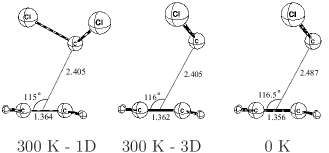
Figure 1: Transition states geometries for the addition of dichlorocarbene CCl_2 to ethylene, optimized at 0K, at 300K with only the $d_{CG}$ distance constrained (1D), and at 300K with $d_{CG}$, $d_{CC}$ and $\alpha$ all constrained (3D). $G$ is the midpoint of the double bond. Distances in Å, angles in deg.

	$d_{CG}$ (Å)	$d_{CC}$ (Å)	$\alpha$ (deg.)
1D	2.405(2)(a)	1.364(2)(b)	115(1)(b)
3D	2.405(2)	1.362(2)	116(1)
0K	2.487	1.356	116.5

Table 1: Main geometrical parameters for the transition state geometries for the addition of the dichlorocarbene CCl_2 on ethylene, optimized at 0K, at 300K with one constraint (1D), and at 300K with three constraints (3D). (a) Estimate of the uncertainty. The uncertainty for structures on the potential energy surface is much smaller, and thus not quoted. (b) Average values.

All three structures are non symmetric: the $\alpha$ angle is approximately equal to 115° instead of 90°. This is in agreement with the Woodward-Hoffman rules and with previous calculationsHRM84 ; BWJ89 ; KYM99 ; BCK04 ; KMSH99 and experimental results.KMSH99 More, all geometries correspond to an early transition state in which the ethylene molecule is only slightly distorted. The double bond length equals approximately 1.36 Å, close to the equilibrium distance in the free molecule: $d_{CC}=1.33$ Å.

The two structures found at 300K are almost identical. This is not surprising: as already stated the distance $d_{CG}$ between the middle of the double bond and the carbon atom of the carbene is a good reaction coordinate up to this point.

The transition state geometry at 0K is in fairly good agreement with previous ab initio calculationsHRM84 ; BWJ89 ; KYM99 ; BCK04 except for the $d_{CG}$ distance which is slightly overestimated here: $d_{CG}=2.487$ Å compared to $d_{CG}=2.37$ Å at the B3LYP/6-31G* level,BCK04 or $d_{CG}=2.38$ Å at the MP2/6-31G* level.BWJ89 ; KYM99 ; BCK04 This is due to the fact that this region of the potential energy surface is shallow so that the location of the transition state depends strongly on the functional and on the basis set used. Similarly, the $\alpha$ angle is also a bit overestimated: it equals 116.5° in our study, whereas it equals respectively 111.7° and 112.2° at the MP2/6-31G* and B3LYP/6-31G* levels of calculation.BWJ89 ; KYM99 ; BCK04

Going from the transition state structure found at 0K to that obtained at 300K leads to an increase of the double bond length due to thermal vibrations. On the other hand, the $d_{CG}$ distance is smaller at hight temperature. This comes from the fact that the barrier originates mainly from rotational entropy lost when the transition state is formed. As the average rotational momentum increases with the temperature, we expect this barrier to move to smaller distance as the temperature rises. This is in agreement with previous studies.KSZ04 ; YHFZ04

IV.1.2 1,1’-dichlorocyclopropane

The main geometrical parameters for the 1,1’-dichlorocyclopropane are reported in Table 2 and the corresponding structures are given in Figure 2. All three structures are very symmetric: $\alpha=90$° which means that the carbon atoms form an isocel triangle, its base being the former ethylenic bond. All three carbon-carbon bond length are now close to that of a single bond: $d_{C^{1}C^{3}}=1.53$ Å, $d_{C^{1}C^{2}}=d_{C^{3}C^{2}}=1.50$ Å.

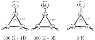
Figure 2: Geometries of the 1,1’-dichloro cyclopropane optimized at 0K, at 300K with only the $d_{CG}$ distance constrained (1D), and at 300K with $d_{CG}$, $d_{CC}$ and $\alpha$ all three constrained (3D). $G$ is the midpoint of the double bond. Distances in Å, angles in deg.

	$d_{CG}$ (Å)	$d_{CC}$ (Å)	$\alpha$ (deg.)
1D	1.289(2)(b)	1.535(2)(b)	90(1)(b)
3D	1.289(2)	1.532(2)	90(1)
0K	1.288	1.527	90.1

Table 2: Main geometrical parameters for the 1,1’-dichlorocyclopropane, optimized at 0K, at 300K with one constraint (1D), and with three constraints (3D). (a) Estimate of the uncertainty. (b) Average values.

Similarly to what was observed for the transition state structures, there are very little difference between the room temperature 1D and 3D structures. This comes from the fact that the gradient is zero for a minimum, so that the definition of the reaction coordinate does not matter anymore. To further assess this point, we have launched a simulation with no constraints. The average values of $d_{CG}$, $d_{CC}$ and $\alpha$ are in very good agreement with the constrained simulations: $d_{CG}=1.291\pm 0.002$ Å, $d_{CC}=1.533\pm 0.002$ Å and $\alpha=90.\pm 1$°.

The 0K structure is in good agreement with previous calculations: the difference in distances and angles is less then 0.01 Å, and 1°, respectively.HRM84 When going from 0K to 300K, the C-C bonds elongate, while $d_{CG}$ and $\alpha$ remain constant. This comes from the fact that this molecule has a C_2v symmetry which imposes that the average angle should be close to its value on the potential energy surface.

IV.2 Reaction Path

We focus now on the core of this application: the construction of the reaction path connecting the reactants to the product, directly on the free energy surface. The aim of this part is dual: first, we show how to use the previous formula on a real example. Second, we compare the 3D path constructed here to the path obtained with only one ‘chemically intuitive’ reaction coordinate. Starting from the transition state, we have constructed the forward reaction path leading to the product and the backward path leading to the reactants.

In this work, we have moved along the gradient employing a small step size: at each point $\mathbf{x^{k}}$ of the path, a simulation is launch while constraining all three active coordinates $d_{CG}$, $d_{CC}$ and $\alpha$. The previous formulas ((98), (99) and (100)) are used to compute the free energy gradient: $\mathbf{g}=\left(\frac{\partial A}{\partial d_{CG}},\frac{\partial A}{\partial d_{CC}},\frac{\partial A}{\partial\alpha}\right)^{t}$. We then convert this gradient into a normalized mass weighted gradient: $\mathbf{g}_{MW}=\mathcal{N}\mathbf{Z_{\xi}}\mathbf{g}$, with $\mathcal{N}=(\mathbf{g}^{t}\mathbf{Z_{\xi}}\mathbf{g})^{\nicefrac{{-1}}{{2}}}$. The next point $\mathbf{x^{k+1}}$ is calculated by following the gradient on a small distance $ds$:

$$\mathbf{x^{k+1}}=\mathbf{x^{k}}-ds\times\mathbf{g}_{MW}$$ (101)

An alternative way is to employ the scheme derived by Gonzalez et al.GS89 which allows for the use of a much bigger stepsize. The forward path corresponds to the closure of the cycle, that is to say to the formation of the second carbon-carbon bond. The gradient along this path is large, and we used a stepsize of 0.5 a.u.footnote1 The backward path corresponds to the departure of the carbene, which is the reverse of the electrophilic addition. The change in free energy is small in that direction, and we had to employ a smaller stepsize of 0.2 a.u. to minimize the statistical noise.

IV.2.1 Free energy profile

The resulting free energy profile (FEP) is reported in Figure 3 together with the profile generated with one constraint.KSZ04 In order to compare them, both paths have been plotted using the $d_{CG}$ distance as an approximate reaction coordinate. The FEP obtained in the present work is given as an inset in Figure 3. The two profiles are very similar: first, the free energy increases smoothly from the isolated reactants to the transition state. Then, it decreases abruptly when the cyclopropane is formed.

On an energetic ground, in agreement with the fact that the free energy is a state function, both path lead to a similar change in free energy equal to: $\Delta A_{corr}$ = -47.6 kcal$\cdot$mol^-1 in this work, and $\Delta A_{corr}$ = -46.5 kcal$\cdot$mol^-1 in our previous work, when employing 40000 steps. More, as $d_{CG}$ is a good reaction coordinate for the first phase, the barrier is also similar in both cases: $\Delta A^{TS}_{corr}\approx$ 11.5 kcal$\cdot$mol^-1 in this work, compared to $\Delta A^{TS}_{corr}\approx$ 11.7 kcal$\cdot$mol^-1 previously. These values are in good agreement with the previous studies.KSZ04 ; BWJ89

Figure 3: Free Energy Profile (FEP) for the addition of dichlorocarbene CCl_2 to ethylene. The 1D profile is calculated using $d_{CG}$ as the predefined reaction coordinate, whereas the 3D profile uses an active set of three coordinates ($d_{CG}$, $d_{CC}$, $\alpha$). The inset shows the FEP plotted against the curvilinear distance from the transition state along the 3D path. $G$ is the midpoint of the double bond.

IV.2.2 Geometrical parameters

Even thought the two free energy profiles are similar, the two path are actually quite different in terms of geometrical parameters. We discuss here the variations of the structural parameters $d_{CC}$ and $\alpha$ for both path. The evolution of the double bond distance $d_{CC}$ and of the $\alpha$ angle obtained in this study are reported on Figure 4 together with the average values $\left<d_{CC}\right>$ and $\left<\alpha\right>$ obtained in the previous study using only $d_{CG}$ as a reaction coordinate.

The first feature worth noting is that the forward path, corresponding to the the formation of the second C-C bond, is not parallel to the $d_{CG}$ axis but acquires contributions along both $d_{CC}$ and $\alpha$. This confirms that an accurate description of this step requires a more complex reaction coordinate than just the $d_{CG}$ distance. As a consequence, despite the fact that $d_{CG}$ varies only from 2.40 Å to 1.29 Å for the second phase, the actual path length is of the same order of magnitude as for the first phase: $s\approx 10$ a.u.

Figure 4: Reaction path for the addition of dichlorocarbene to ethylene. Two projections are show: in the $d_{CC}-d_{CG}$ and $\alpha-d_{CG}$ subspace, $G$ being the midpoint of the double bond. The 1D path is obtained using $d_{CG}$ as the reaction coordinate, whereas the 3D path uses an active set of three coordinates ($d_{CG}$, $d_{CC}$, $\alpha$).

The evolution of the two structural parameters $d_{CC}$ and $\alpha$ can be divided into three zones. The first one corresponds to $d_{CG}\gtrsim 2.6$ Å. In this zone, there is little interaction between the two reactants: $d_{CC}$ is constant and equal to 1.33 Å, which is the standard double bond length, and $\alpha$ tends to 90°.footnote2 This comes from the fact that, for the unconstrained system, at large separation there is free rotation of the carbene around the ethylene molecule. As a consequence, $\alpha$ should vary freely between 0° and 180°, with an average value of 90°.

The second zone corresponds to the electrophilic addition, that is the formation of the first bond between the carbene and the ethylene molecule. In this zone, $d_{CG}$ evolves from ca. 1.8 Å to ca. 2.6 Å. As the two molecules start to interact the ethylenic bond elongates from 1.33 Å to ca. 1.48 Å. As expected, this last value is intermediate between a single and a double carbon-carbon bond length. Simultaneously, $\alpha$ increases to 128°. This is a consequence of the fact that the symmetric approach for which $\alpha=90$° is forbidden, and is thus associated with a very high barrier.KMSH99 During this phase, the $C^{1}C^{2}$ bond is formed: this distance decreases from 2.4 Å to 1.56 Å, which is close to a single bond.

The last zone corresponds to $d_{CG}\leq 1.8$ Å and represents the closure of the cyclopropane ring. The $C^{1}C^{3}$ bond (formerly the double bond) length increases to its finals value of 1.538 Å, while $\alpha$ drops to 90°. Comparing the path constructed using a 3 coordinates active space to the path previously obtained shows that $\alpha$ is a much better reaction coordinate for this phase than $d_{CG}$. Indeed, during this phase the $C^{1}C^{2}$ distance is almost constant and close to 1.54 Å, while the $C^{3}C^{2}$ distance decreases strongly from 2.3 Å to 1.54 Å. This illustrates that the second phase of the reaction is actually the bending of the $C^{1}C^{2}$ bond towards the $C^{3}$ carbon atom. For this type of movement $\alpha$ is a good reaction coordinate whereas $d_{CG}$ is a poor one. As a consequence, when only $d_{CG}$ is used as a reaction coordinate, $\alpha$ drops abruptly from 115° to 90° around $d_{CG}=1.36$ Å. On the other hand, the variations of $\alpha$ are much smoother with our active set.

To conclude this section, we would like to point out that, as expected, both path are qualitatively similar, with the same overall evolutions of the geometrical parameters. However, they differ significantly on a quantitative basis, especially in the third zone. This is due to the fact that $d_{CG}$ is not a good approximation to the reaction coordinate in this zone. To illustrate how this explains why the two path are different, let us consider a force acting on the $d_{CC}$ variable at the point A (Fig. 4) located in this zone. We denote the local coordinate set by $(\xi,u,v)$, with $\xi$ being the reaction coordinate. From the definition of a reaction coordinate, we have:

$$\frac{\partial A}{\partial\xi}=g\not=0$$ (102)

$$\frac{\partial A}{\partial u}=0$$ (103)

$$\frac{\partial A}{\partial v}=0$$ (104)

As $d_{CG}$ is not a good approximation to the reaction coordinate, $\xi$ depends not only on $d_{CG}$ but also on $d_{CC}$ and $\alpha$. As a result, the derivative of the free energy along $d_{CC}$ is related to the gradient of the free energy:

$$\frac{\partial A}{\partial d_{CC}} =\frac{\partial A}{\partial\xi}\frac{\partial\xi}{\partial d_{CC}}+\frac{\partial A}{\partial u}\frac{\partial u}{\partial d_{CC}}+\frac{\partial A}{\partial v}\frac{\partial v}{\partial d_{CC}}$$

$$=\frac{\partial A}{\partial\xi}\frac{\partial\xi}{\partial d_{CC}}\not=0$$ (105)

Thus, if $d_{CC}$ is not constrained, the system will evolve in order to minimize the free energy in that direction, and the two paths will not coincide.

IV.3 Importance of the correction to evaluate the gradients

It is worth analyzing the importance of the B terms in equations (98)-(100). They are reported on Figure 5 together with the average value of the Lagrange multipliers. It appears that those terms are usually smaller than the Lagrange multiplier by at least an order of magnitude. However, as the reaction path is following the free energy gradient, these small differences are accumulated along the path, leading to a non-negligible correction. For example, for the studied reaction, the free energy correction along the path can reach 1 kcal$\cdot$mol^-1. The larger correction for the geometrical parameters is observed for the evolution of the double bond length: $\Delta(d_{CC})\approx 0.01$ Å. However, the structural differences for the product and the transition state are much smaller: $\Delta(d)\leq 0.005$ Å and $\Delta(\alpha)\leq 0.5$°. The correction for the total free energy difference is only $\Delta(\Delta A_{corr})=0.1$ kcal$\cdot$mol^-1.

Figure 5: Importance of the correction terms in the evaluation of the free energy derivative. $\left<\lambda_{X}\right>$ is the average of the Lagrange multiplier. $B_{CG}=-kT\frac{Z_{d_{CG}}}{Z_{\alpha}d^{3}_{CG}}$ and $B_{CC}=-kT\frac{Z_{d_{CC}}}{Z_{\alpha}d^{3}_{CC}}$ are the correction to the derivative of the free energy along $d_{CG}$ and $d_{CC}$ respectively. $G$ is the midpoint of the double bond.

We would like to draw attention to the fact that, even thought those terms are generally not negligible, one should not forget that we are using classical mechanics, and that all quantum effects are missing for the description of the nuclei motion. In particular, ZPE and tunneling are completely neglected.

IV.4 Effect of the temperature

Following the procedure of Gonzalez et al.,GS89 we have constructed the reaction path at 0K. As the differences between the potential energy profile and the free energy profile have already been discussed,KSZ04 we shall focus here on the differences between the path at 0K and 300K. The two path are reported on figure 6.

Figure 6: Reaction path for the addition of the dichlorocarbene to ethylene at 0K and 300K. Two projections are show: in the $d_{CC}-d_{CG}$ and $\alpha-d_{CG}$ subspace, $G$ being the midpoint of the double bond.

At large separation, that is for the electrophilic addition, $d_{CG}$ is a good reaction coordinate at both temperatures. More, as long as the two reactants interact only weakly, the thermal motions are mainly vibrations of the two molecules. As the potential energy surface is almost harmonic for such vibrations, the evolutions of the double bond distance and of the angle $\alpha$ are similar at 300K and at 0K. On the potential energy surface, as the distance between the two fragments increases, the interaction depends less and less on the angle, leading to some spurious evolutions. On the free energy surface, this independence of the interaction on the angle leads to an average value of 90° instead.

When the interaction starts to be stronger, these oscillations of the angle disappear and both path are qualitatively similar. However, due to the vibrational thermal energy, at 300K the parameters changes are larger.

IV.5 Computational details

The Car-Parrinello projector augmented-wave (CP-PAW)PAW1 ; PAW2 program by Blöchl was used for all AIMD calculations. In the CP-PAW calculations, periodic boundary conditions were used in all examples with an orthorhombic unit cell described by the lattice vectors ([0, 14.74, 14.74], [14.74, 0, 14.74], [14.74, 14.74, 0]) (bohr, 7.8 Å). The energy cutoff used to define the basis set was 30 Ry (15 a.u.) in all cases. Because the systems of interest are all isolated molecules, only the $\Gamma$-point in k-space was included and the interaction between images was removed by the method proposed by Blöchl.PAW2 The approximate density-functional theory (DFT) used here consisted of the combination of the Perdew-Wang parametrization of the electron gasPW91 in combination with the exchange gradient correction presented by BeckeB88 and the correlation correction of Perdew.PExc The SHAKE algorithmSHAKE was employed in order to impose the constraints. The mass of the hydrogen atoms was taken to be that of deuterium, and normal masses were taken for all other elements.

Room temperature CP-PAW calculations were performed at a target temperature of 300 K. The Andersen thermostatAndersen80 was applied to the nuclear motion by reassigning the velocity of N randomly chosen nuclei every n steps where N and n are chosen to maintain the desired temperature. In our case this amounted to one velocity reassignment every 20 steps. Thermostat settings were monitored and adjusted if necessary during the equilibration stage, with the main criteria for adequate thermostating being the mean temperature lying within a range of $300\pm 10$ K and a temperature drift lower than 1 K/ps. In combination with the Andersen thermostat, a constant friction was applied to the wave function with a value of 0.001. Following the conclusions of the previous study, for each simulation, we performed between 35000 and 50000 steps in order to ensure that the system was fully equilibrated and that the temperature and the free energy gradient were fully converged.

The free energy profiles were obtained by numerical integration of the gradient along the path, using a procedure similar to the pointwise thermodynamic integration (PTI) method.SC91 As the overall rotation and translation of the molecule are frozen during a simulation, one has to correct the free energy obtained from a simulation. We have used the procedure of Kelly et al.KSZ04 To summarize, the overall correction for the entropy is the sum of the translational and rotational entropy:

$$\Delta S^{AB}_{corr}(s)=S_{R}^{AB}(s)+S_{T}^{AB}(s)-S_{T}^{A}(\infty)-S_{T}^{B}(\infty)$$ (106)

Where $S_{R}^{AB}(s)$ is the rotational entropy at RC = s which is geometry dependent, and $S_{T}^{AB}(s)$ is the translational entropy at RC =s. The last two terms represent the translational entropy of the isolated species A and B. These terms are calculated using standard formula for the partition functions. Finally, the total free energy change $\Delta A^{AB}_{corr}(s)$ is obtained from a CP-PAW simulation with the constraints described above as

$$\Delta A^{AB}_{CM}(s)=\Delta A^{AB}_{PAW}(s)-T\Delta S^{AB}_{corr}(s)$$

where $\Delta A^{AB}_{PAW}(s)$ is the change in free energy obtained directly from the simulation, and CM (classical mechanics) refers to the fact that the motion of the nuclei is described using classical mechanics. It should be mentioned that the zero-point energy (ZPE) correction is not included in our simulations. This should not seriously hamper our objective which is to analyze the qualitative differences between the path obtained with one and three constraints.

V Conclusion

In this work, we have proposed a new look at the standard formulas for evaluating the derivatives of the free energy along a reaction coordinate.

First, we recollected the different formulas available in a uniform approach. These formulas allow one to compute accurately and efficiently the gradient of the free energy for an unconstrained system using a constrained molecular dynamic simulation.

The main finding of this investigation is a set of equations that makes it possible to construct a minimum free energy reaction path instead of calculating the free energy changes along a predefined path. Indeed, we believe that one can use the free energy gradients in the same way potential energy gradients have been used in the past 20 years in quantum chemistry calculations.

Addition of the dichlorocarbene to ethylene was studied as a numerical example. It was shown that a simulation using only one constraint is not sufficient to describe the whole path. Using the free energy gradient in a subset of three active coordinates lead to a smoother path, refining the understanding of this process.

Appendix A Properties of the Mass matrix

Using $\mathbf{A}_{q\xi}^{-1}\mathbf{A}_{q\xi}=\mathbf{I}$, one readily finds:

$$\mathbf{X}_{q}\mathbf{A}_{q}+\mathbf{Y}_{\xi}\mathbf{B_{\xi}}^{t} =\mathbf{I_{3N-1}}$$ (107)

$$\mathbf{X}_{q}\mathbf{B_{\xi}}+\mathbf{Y_{\xi}}C_{\xi} =\mathbf{0}$$ (108)

$$\mathbf{Y}_{\xi}^{t}\mathbf{A}_{q}+Z_{\xi}\mathbf{B}_{\xi}^{t} =\mathbf{0}$$ (109)

$$\mathbf{Y}_{\xi}^{t}\mathbf{B_{\xi}}+Z_{\xi}C_{\xi} =1$$ (110)

Plugging equation (109) into equation (107) leads to

$$\mathbf{A}_{q}^{-1}=\mathbf{X}_{q}-\mathbf{Y_{\xi}}Z_{\xi}^{-1}\mathbf{Y}_{\xi}^{t}$$ (111)

The last relation we need derives from:

$$\left(\begin{array}[]{cc}\mathbf{A}_{q}&\mathbf{0}\\ \mathbf{B}_{\xi}^{t}&1\\ \end{array}\right)=\mathbf{A}_{q\xi}\mathbf{A}_{q\xi}^{-1}\left(\begin{array}[]{cc}\mathbf{A}_{q}&\mathbf{0}\\ \mathbf{B}_{\xi}^{t}&1\\ \end{array}\right)=\mathbf{A}_{q\xi}\left(\begin{array}[]{cc}\mathbf{I}_{3N-1}&\mathbf{Y}_{\xi}\\ \mathbf{0}&Z_{\xi}\\ \end{array}\right)$$ (112)

Equating the determinant of the first and last term, we get:

$$\mid\mathbf{A}_{q\xi}\mid=\mid\mathbf{A}_{q}\mid\mid Z_{\xi}\mid^{-1}=\mid\mathbf{J}^{t}\mathbf{M}\mathbf{J}\mid=\mid\mathbf{J}\mid^{2}\mid\mathbf{M}\mid$$ (113)

Appendix B Properties of Gaussian integrals

We recall here the main properties of Gaussian integrals:

$$\int\mathbf{du}e^{\left(-\mathbf{u}^{t}\mathbf{A}\mathbf{u}\right)} \propto\mid\mathbf{A}\mid^{-\nicefrac{{1}}{{2}}}$$ (114)

$$\int\mathbf{du}e^{\left(-\mathbf{u}^{t}\mathbf{A}\mathbf{u}\right)}\mathbf{u}^{t}\mathbf{B}\mathbf{u} \propto\frac{1}{2}\text{Tr}\left(\mathbf{A}^{-1}\mathbf{B}\right)\int\mathbf{du}e^{\left(-\mathbf{u}^{t}\mathbf{A}\mathbf{u}\right)}$$ (115)

Appendix C Constraining the overall rotation and translation

In this section, we derive the expressions used to constrain the overall translation and rotation of the system. For this, we start from a reference geometry $\mathbf{x^{0}}$ and we seek the conditions that should be satisfied by the new geometry $\mathbf{x}$. The Center of Mass G is defined by:

$$\mathbf{x_{G}}=\frac{\sum_{i=1}^{N}m_{i}\mathbf{x_{i}}}{\sum_{i=1}^{N}m_{i}}$$

where $m_{i}$ is the mass of the atom $i$ with coordinate $\mathbf{x_{i}}$. In the following, the notation $\widetilde{\mathbf{x}}_{i}=\mathbf{x_{i}}-\mathbf{x_{G}}$ will be used. Let us denote by $\hat{x}$, $\hat{y}$ and $\hat{z}$ the unit vectors of our laboratory coordinate system. For the sake of clarity, the component of $x_{i}$ along the $\hat{x}$, $\hat{y}$ and $\hat{z}$ axis will be denoted by $x_{i,1}$, $x_{i,2}$ and $x_{i,3}$ respectively.

Constraining the translation is equivalent to freeze the movement of the center of mass, i.e. to apply the following linear constraints:

$$\sigma_{1}=\sum_{i=1}^{N}\frac{m_{i}}{M}\left(x_{i,1}-x^{0}_{i,1}\right)=0$$ (116a)

$$\sigma_{2}=\sum_{i=1}^{N}\frac{m_{i}}{M}\left(x_{i,2}-x^{0}_{i,2}\right)=0$$ (116b)

$$\sigma_{3}=\sum_{i=1}^{N}\frac{m_{i}}{M}\left(x_{i,3}-x^{0}_{i,3}\right)=0$$ (116c)

Constraining the rotation can be done by using the second Eckart conditions.Eckart35 These conditions minimize the angular momentum due to small displacements: they provide an approximate way to constrain the global rotation during a molecular dynamic simulation:

$$\sigma_{4}=\hat{x}\cdot\left[\sum_{i=1}^{N}m_{i}\left(\widetilde{\mathbf{x}^{0}_{i}}\times\widetilde{\mathbf{x_{i}}}\right)\right]=0$$ (117a)

$$\sigma_{5}=\hat{y}\cdot\left[\sum_{i=1}^{N}m_{i}\left(\widetilde{\mathbf{x}^{0}_{i}}\times\widetilde{\mathbf{x_{i}}}\right)\right]=0$$ (117b)

$$\sigma_{6}=\hat{z}\cdot\left[\sum_{i=1}^{N}m_{i}\left(\widetilde{\mathbf{x}^{0}_{i}}\times\widetilde{\mathbf{x_{i}}}\right)\right]=0$$ (117c)

that is:

$$\sigma_{4}=\sum_{i=1}^{N}m_{i}\left(\widetilde{x}^{0}_{i,2}\widetilde{x}_{i,3}-\widetilde{x}_{i,2}\widetilde{x}^{0}_{i,3}\right)=0$$ (118a)

$$\sigma_{5}=\sum_{i=1}^{N}m_{i}\left(\widetilde{x}^{0}_{i,3}\widetilde{x}_{i,1}-\widetilde{x}_{i,3}\widetilde{x}^{0}_{i,1}\right)=0$$ (118b)

$$\sigma_{6}=\sum_{i=1}^{N}m_{i}\left(\widetilde{x}^{0}_{i,1}\widetilde{x}_{i,2}-\widetilde{x}_{i,1}\widetilde{x}^{0}_{i,2}\right)=0$$ (118c)

These last equations can be written as linear constraints:

$$\sigma_{4}=\sum_{i=1}^{N}m_{i}\left\{x_{i,3}\left(\widetilde{x}^{0}_{i,2}-\sum_{j=1}^{N}\frac{m_{j}}{M}\widetilde{x}^{0}_{j,2}\right)-x_{i,2}\left(\widetilde{x}^{0}_{i,3}-\sum_{j=1}^{N}\frac{m_{j}}{M}\widetilde{x}^{0}_{j,3}\right)\right\}=0$$ (119a)

$$\sigma_{5}=\sum_{i=1}^{N}m_{i}\left\{x_{i,1}\left(\widetilde{x}^{0}_{i,3}-\sum_{j=1}^{N}\frac{m_{j}}{M}\widetilde{x}^{0}_{j,3}\right)-x_{i,3}\left(\widetilde{x}^{0}_{i,1}-\sum_{j=1}^{N}\frac{m_{j}}{M}\widetilde{x}^{0}_{j,1}\right)\right\}=0$$ (119b)

$$\sigma_{6}=\sum_{i=1}^{N}m_{i}\left\{x_{i,2}\left(\widetilde{x}^{0}_{i,1}-\sum_{j=1}^{N}\frac{m_{j}}{M}\widetilde{x}^{0}_{j,1}\right)-x_{i,1}\left(\widetilde{x}^{0}_{i,2}-\sum_{j=1}^{N}\frac{m_{j}}{M}\widetilde{x}^{0}_{j,2}\right)\right\}=0$$ (119c)

Appendix D Actually calculating eq. 59

In this appendix, we propose one way to calculate the derivatives of the free energy A along $q_{n}$, using a simulation in which only $\xi$ is constrained. As an example, we consider that the coordinates $q_{i}$ to $q_{n}$ were inactive at step $k-1$ and become active at step $k$.

The first step is to use the expressions for the generalized coordinates to obtain the values for $\mathbf{Z_{\xi}}$, $Z_{q_{n}}$, $\frac{\partial Z_{q_{n}}}{\partial x^{\prime}}$ and $\frac{\partial q_{n}}{\partial x^{\prime}}$.

The main difficulty in using equation (59) is that one must ensure that the sampling of $q_{n}$ around $q_{n}^{k}$ is sufficient. In practice, this imposes to have long MD simulations, with approximately 100000 steps for each considered inactive coordinate. One way to circumvent this problem is to use a Taylor expansion of the derivative of the potential around $q_{i}^{k}$, …, $q_{n}^{k}$:

$$\frac{\partial V}{\partial q_{n}}=\left.\frac{\partial V}{\partial q_{n}^{k}}\right)_{q_{i}^{k},\ldots,q_{n}^{k},\xi^{*}}+\sum_{j=i}^{j=n}\left.\frac{\partial^{2}V}{\partial q_{n}\partial q_{j}}\right)_{q_{i}^{k},\ldots,q_{n}^{k},\xi^{*}}(q_{j}-q_{j}^{k})\\ +\frac{1}{2}\left.\sum_{j=i}^{j=n}\sum_{l=i}^{l=n}\frac{\partial^{3}V}{\partial q_{n}\partial q_{j}\partial q_{l}}\right)_{q_{i}^{k},\ldots,q_{n}^{k},\xi^{*}}(q_{j}-q_{j}^{k})(q_{l}-q_{l}^{k})$$ (120)

The simulation data is then used to fit the coefficients of this expression. The resulting equation is then plugged into equation (59).

References

- (1) M. P. Allen and D. J. Tildesley, Computer Simulation of Liquids (Clarendon, Oxford, England, 1987).
- (2) C. Chipot and D. A. Pearlman, Mol. Simul. 28, 1 (2002), and references therein.
- (3) S. Park and K. Schulten, J. Chem. Phys. 120, 5946 (2004).
- (4) F. M. Ytreberg and D. M. Zuckerman, J. Chem. Phys. 120, 10876 (2004).
- (5) C. Jarzynski, Phys. Rev. Let. 78, 2690 (1997).
- (6) C. Jarzynski, Phys. Rev. E 56, 5018 (1997).
- (7) R. W. Zwanzig, J. Chem. Phys. 22, 1420 (1954).
- (8) G. M. Torrie and J. P. Valleau, J. Comput. Phy. 23, 187 (1977).
- (9) T. P. Straatsma and J. A. McCammon, J. Chem. Phys. 95, 1175 (1991).
- (10) W. F. van Gunsteren, in Computer Simulations of Biomolecular Systems: Theoretical and Experimental Applications, edited by W. F. van Gunsteren and P. K. Weiner, vol. 1, page 27 (ESCOM, Leiden, The Netherlands, 1989).
- (11) E. A. Carter, G. Ciccotti, J. T. Hynes, and R. Kapral, Chem. Phys. Letters 156, 472 (1989).
- (12) M. Sprik and G. Ciccotti, J. Chem. Phys. 109, 7737 (1998).
- (13) W. K. den Otter and W. J. Briels, J. Chem. Phys. 109, 4139 (1998).
- (14) E. Darve and A. Pohorille, J. Chem. Phys. 115, 9169 (2001).
- (15) K. Fukui, J. Phys. Chem. 74, 4161 (1970).
- (16) K. Fukui, Acc. Chem. Res. 14, 363 (1981).
- (17) W. K. den Otter and W. J. Briels, Mol. Phys. 98, 773 (2000).
- (18) E. Darve, M. A. Wilson, and A. Pohorille, Mol. Simul. 28, 113 (2002).
- (19) J. Schlitter and M. Klähn, Mol. Phys. 101, 3439 (2003).
- (20) J.-P. Ryckaert, G. Ciccotti, and H. J. C. Berendsen, J. Comput. Phys. 23, 327 (1977).
- (21) G. Vilasi, Hamiltonian Dynamics, chap. 2, page 45 (World Scientific Publishing Co. Pte. Ltd., London, England, 2001).
- (22) J. Schlitter, W. Swegat, and T. Mülders, J. Mol. Model. 7, 171 (2001).
- (23) E. B. Wilson, Jr., J. C. Decius, and P. C. Cross, Molecular Vibrations (McGraw Hill Book Company, 1955).
- (24) A. Michalak and T. Ziegler, J. Phys. Chem. A 105, 4333 (2001).
- (25) E. Kelly, M. Seth, and T. Ziegler, J. Phys. Chem. A 108, 2167 (2004).
- (26) N. G. Rondam, K. N. Houk, and R. A. Moss, J. Am. Chem. Soc. 102, 1770 (1980).
- (27) K. Krogh-Jespersen, S. Yan, and R. A. Moss, J. Am. Chem. Soc. 121, 6269 (1999).
- (28) H. B. Schlegel, in Encyclopedia of Computational Chemistry, edited by P. v. R. Schleyer, N. L. Allinger, T. Clark, J. Gasteiger, P. A. Kollman, H. F. Schaefer III, and P. R. Schreiner, page 1136 (Wiley, Chichester, 1998), and references therein.
- (29) J. M. Bofill, J. Comput. Chem. 15, 1 (1994).
- (30) S. Yang, I. Hristov, P. Fleurat-Lessard, and T. Ziegler, J. Phys. Chem. A 109, 197 (2005).
- (31) K. N. Houk, N. G. Rondam, and J. Mareda, J. Am. Chem. Soc. 106, 4291 (1984).
- (32) J. F. Blake, , S. G. Wiershke, and W. L. Jorgensen, J. Am. Chem. Soc. 111, 1919 (1989).
- (33) J. J. Blavins, D. L. Cooper, and P. B. Karadakov, Int. J. Quantum Chem. 98, 465 (2004).
- (34) A. E. Keating, S. R. Merrigan, D. A. Singleton, and K. N. Houk, J. Am. Chem. Soc. 121, 3933 (1999).
- (35) C. Gonzalez and H. B. Schlegel, J. Chem. Phys. 90, 2154 (1989).
- (36) Even thought this value might seem quite large, because of the two heavy chlorine atoms, a step of 0.5 a.u. corresponds to a decrease of the distance by approximately 0.005 Å only.
- (37) The convergence is slow, and is not shown on the figure.
- (38) P. E. Blöchl, Phys. Rev. B 50, 17953 (1994).
- (39) P. E. Blöchl, J. Phys. Chem. 99, 7422 (1995).
- (40) J. P. Perdew and Y. Wang, Phys. Rev. B 45, 13244 (1992).
- (41) A. Becke, Phys. Rev. A 38, 3098 (1988).
- (42) J. P. Perdew, Phys. Rev. B 33, 8822 (1986).
- (43) H. C. Andersen, J. Chem. Phys. 72, 2384 (1980).
- (44) C. Eckart, Phys. Rev. 47, 552 (1935).