Synchrotron dynamics in Compton x-ray ring with nonlinear momentum compaction

Abstract

The longitudinal dynamics of electron bunches with a large energy spread circulating in the storage rings with a small momentum compaction factor is considered. Also the structure of the longitudinal phase space is considered as well as its modification due to changes in the ring parameters. The response of an equilibrium area upon changes of the nonlinear momentum compaction factor is presented.

I Introduction

Engagement of electron storage rings for production of x rays through Compton scattering of laser photons against ultrarelativistic electrons was proposed in 1998 Huang and Ruth (1998). Two basic schemes exist so far. One of them supposes use of electron beams with unsteady parameters Loewen (2003) and applies the continual injection (and ejection of circulating bunches by the next injecting pulse) of dense intensive bunches. The second scheme is based on the continuous circulation of bunches. To make the bunches acquired a sufficiently large energy spread confined (see Bulyak (2004)), a lattice with a small controllable momentum compaction factor is proposed to employ Crooker et al. (2005). The longitudinal dynamics in the small compaction lattice is governed not only by the linear effects of the momentum deviation but by the nonlinear ones as well.

In Compton sources storing the bunches with the large energy spread which can be as high as a few percents, ring’s energy acceptance becomes compared to the energy spread. To get proper life time of the circulating electrons, the energy acceptance $\sigma\equiv\max(E-E_{s})/E_{s}$ ($E_{s}$ is the energy of synchronous particle) should be high enough.

Within a linear approximation according to the energy deviation, the acceptance can be increased either by enhancement of the RF voltage, $V_{\mathrm{rf}}$, or by decreasing of the linear momentum compaction factor $\alpha_{0}$ since $\sigma\propto\sqrt{V_{\mathrm{rf}}/\alpha_{0}}$.

The paper presents results of study on the longitudinal dynamics of electron bunches circulating in storage rings with a small linear momentum compaction factor $\alpha_{0}$. Structure of the phase space are considered and its deformation with changes in the ring lattice parameters. In particular, the size of stable area as a function of the RF voltage and momentum compaction is evaluated.

II Finite-difference model of longitudinal motion

Let us consider a model of the ring comprised only two components: drift and radio frequency (rf) cavity. For the sake of simplicity we will suggest the cavity infinitely short, in which the particle momentum (energy) suffer an abrupt change while the phase of a particle remains unchanged. On the contrary, the phase of a particle traveling along the drift changes while the energy remains invariable. The longitudinal motion in a such idealized ring will be described in canonically conjugated variables $\phi$ (the phase about zero voltage in the cavity) and the momentum $p\equiv(\gamma-\gamma_{s})/\gamma_{s}$ equal to the relative deviation of the particle energy from the synchronous one ($\gamma_{s}$ is the Lorentz factor of the synchronous particle).

To study systems able to confine the beams with large energy spread, one needs to account not only the linear part of the orbit deviation from the synchronous one, but nonlinear terms as well:

$$\Delta x\approx D_{1}p+D_{2}p^{2}+\dots\;,$$ (1)

where $D_{1}$ and $D_{2}$ are the dispersion functions of the first and second orders, respectively.

Accordingly, relative lengthening of a (flat) orbit is

$$\frac{\Delta L}{L_{0}} =\oint\sqrt{\left(1+\frac{\Delta x}{\rho}\right)^{2}+\left(\frac{\,\mathrm{d}\Delta x}{\,\mathrm{d}s}\right)^{2}}\,\mathrm{d}s$$

$$\approx\alpha_{0}p+\alpha_{1}p^{2}+\dots\;,$$ (2)

where $L_{0}$ is the length of synchronous orbit, $\rho(s)$ the local radius of curvature, $s$ the longitudinal coordinate. The coefficients $\alpha_{0}$ and $\alpha_{1}$ are determined as

$$\alpha_{1} =\frac{1}{L_{0}}\oint\frac{D_{1}}{\rho}\,\mathrm{d}s\;;$$ (3a)

$$\alpha_{2} =\frac{1}{L_{0}}\oint\left(\frac{D^{\prime 2}_{1}}{2}+\frac{D_{2}}{\rho}\right)\,\mathrm{d}s\;.$$ (3b)

In accordance with the definitions for $\alpha_{0}$ and $\alpha_{1}$, the momentum compaction factor $\alpha_{c}$ can be written as

$$\alpha_{c}=\frac{1}{L_{0}}\frac{\,\mathrm{d}L}{\,\mathrm{d}\delta}\approx\alpha_{0}+2\alpha_{1}p+\dots\;.$$ (4)

To study the phase dynamics in a storage ring with small momentum compaction factor $\alpha_{0}$, the next terms of expansion of the compaction over the energy deviation should be accounted for, hence — the higher terms in the sliding factor $\eta$ Pellegrini and Robin (1991); Lin and da Silva (1993); Feikes et al. (2004). Magnitude of $\eta$ characterizes a relative variation of the phase due to changes of the particle velocity and orbit length. It is determined by the relation

$$\frac{\Delta\phi}{\phi}=\eta(p)p\approx(\eta_{0}+\eta_{1}p+\dots)p\;,$$ (5)

with $\eta_{0}$ and $\eta_{1}$ having been determined by

$$\eta_{0} =\alpha_{0}-1/\gamma^{2}_{s}$$ (6a)

$$\eta_{1} =\alpha_{1}+\eta_{0}+\frac{3}{2\gamma^{2}_{s}}\left(1-\frac{1}{\gamma^{2}_{s}}\right)\;.$$ (6b)

The finite-difference equations for the phase $\phi$ and the variation of relative energy $p$ in the model under consideration read

$$\phi_{f} =\phi_{i}+(\kappa_{0}p_{i}+\kappa_{1}p_{i}^{2})\Delta\tau\;;$$ (7a)

$$p_{f} =p_{i}-U_{\mathrm{rf}}\sin\phi_{f}\Delta\tau\;,$$ (7b)

where

$$\Delta\tau=\tau_{f}-\tau_{i}=\frac{\beta c}{L}(t_{f}-t_{i})\;,$$

the subscripts $i$ and $f$ correspond to the initial and final values, respectively. The dimensionless variable $\tau=t\beta c/L$ represents time expressed in number of rotations ($t$ is time, $\beta c$ the velocity of a particle). The factors $\kappa_{0}$ and $\kappa_{1}$ at a large $\gamma_{s}$ are determined by the expressions $\kappa_{0}=2\pi h\eta_{0}\approx 2\pi h\alpha_{0}$, $\kappa_{1}=2\pi h\eta_{1}\approx 2\pi h(\alpha_{0}+\alpha_{1})$ ( $h$ the harmonic number).

From Eqs. (7), differential (smoothed) equations can be deduced. As it seen, the RHS of (7b) contains the final value of the phase $\phi_{f}$ expressed via the initial value $\phi_{i}$ and momentum $p_{i}$ by the equation (7a).

Let us expand $\sin\phi_{f}$ into series of powers of $\Delta\tau$:

$$\sin\phi_{f} =\sin\left[\phi_{i}+(\kappa_{0}p_{i}+\kappa_{1}p_{i}^{2})\Delta\tau\right]\;$$

$$\approx\sin\phi_{i}+\cos\phi_{i}(\kappa_{0}p_{i}+\kappa_{1}p_{i}^{2})\Delta\tau\;.$$ (8)

Since $\Delta\tau$ can not be regarded as infinitesimal (formally Eqs. (7) present a complete turn, $\Delta\tau=1$), then the linear term can be neglected if $\kappa_{0}p_{i}+\kappa_{1}p_{i}^{2}\ll 1$. In the considered case it can be done since maximum of the energy spread does not exceed a few percents, and the momentum compaction factor $\alpha_{0}$ supposed small. From these assumptions, finite difference equations reduce to

$$\frac{\Delta\phi}{\Delta\tau} =\kappa_{0}p_{i}+\kappa_{1}p_{i}^{2}\;;$$ (9a)

$$\frac{\Delta p}{\Delta\tau} =-U_{\mathrm{rf}}\sin\phi_{i}\;.$$ (9b)

III Differential model of motion

Noting of formal similarity of Eqs. (II) to canonical Hamilton equations describing a mathematical pendulum, we can use a smoothed analog to these equations (a differential substitute for a finite difference equation, $\Delta\tau\to 0$) to facilitate analysis of the motion

$$\frac{\,\mathrm{d}\phi}{\,\mathrm{d}\tau} =\kappa_{0}p+\kappa_{1}p^{2}\;;$$ (10a)

$$\frac{\,\mathrm{d}p}{\,\mathrm{d}\tau} =-U_{\mathrm{rf}}\sin\phi\;.$$ (10b)

A Hamilton function for (10) possesses a specific form with the cubic canonical momentum term

$$H=\frac{\kappa_{1}}{3}p^{3}+\frac{\kappa_{0}}{2}p^{2}+U_{\mathrm{rf}}(1-\cos\phi)\;.$$ (11)

To analyze a phase portrait of the system, it is expedient to present Hamilton function of the longitudinal motion in the reduced form:

$$\tilde{H}=\mu\frac{\tilde{p}^{3}}{3}+\frac{\tilde{p}^{2}}{2}+1-\cos\phi\;,$$ (12)

where

$$\tilde{p} =\sqrt{\frac{\kappa_{0}}{U_{\mathrm{rf}}}}p=\sqrt{\frac{2\pi h\alpha_{0}\gamma_{s}E_{0}}{eV}}p\;;$$ (13a)

$$\mu^{2} =\frac{\kappa^{2}_{1}U_{\mathrm{rf}}}{\kappa^{3}_{0}}=\frac{(\alpha_{0}+\alpha_{1})^{2}eV}{2\pi h\alpha^{3}_{0}\gamma_{s}E_{0}}\;.$$ (13b)

Phase portraits of motion with the Hamiltonian (12) represented in Fig. 1. Topology of the phase plane is governed by the magnitude and sign of the parameter $\mu$. At zero value, $\mu=0$, the Hamiltonian (11) or (12) has a form of mathematical pendulum; its phase plane is presented in Fig. 1(a).

Within the interval $0\leq\mu^{2}<1/12$, there an additional area of finite motion appears; this area is separated from the main area with the band of infinite motion as depicted in Fig. 1(b). When the parameter $\mu$ exceeds the critical value $\mu^{2}_{c}=1/12$ [see Fig. 1(c)], e.g. $1/12\leq\mu^{2}<\infty$, the structure of the phase plane will have changed as is represented in Fig. 1(d).

The dimension of a stable (finite) longitudinal motion, i.e., the area comprised by a separatrix, is in direct proportion with ratio of the ring parameters. For the considered case of the nonlinear Hamiltonian (12), the separatrix height (size along the $p$ axis) is determined by

$$\Delta p =\frac{\alpha_{0}}{\alpha_{0}+\alpha_{1}}\left[\cos\frac{\xi}{3}+\cos\left(\frac{\xi}{3}+\frac{\pi}{3}\right)\right]\;,$$ (14a)

$$\cos\xi=12U_{\mathrm{rf}}\frac{\left(\alpha_{0}+\alpha_{1}\right)^{2}}{\pi h\alpha^{3}_{0}}-1\;,$$

$$\Delta p =\frac{3}{2}\frac{\alpha_{0}}{\alpha_{0}+\alpha_{1}}\;,$$ (14b)

for $\mu\leq\mu_{c}$ (14a) and $\mu\geq\mu_{c}$ (14b), respectively.

Figure 1: Phase portrait of longitudinal motion with account for the cubic nonlinearity at different values of the parameter $\mu$. (a): $\mu=0$, (b): $\mu\leq\left|\mu_{c}\right|$, (c): $\mu=\mu_{c}$, (d): $\mu\geq\left|\mu_{c}\right|$

The phase width of the separatrix (dimension along the $\phi$ axis) is determined by expressions

$$\Delta\phi =2\pi\;;\qquad\mu\leq\mu_{c}\;,$$ (15a)

$$\Delta\phi =2\arccos\left[1-\frac{\pi h}{3U_{\mathrm{rf}}}\frac{\alpha^{3}_{0}}{\left(\alpha_{0}+\alpha_{1}\right)^{2}}\right]\;;$$ (15b)

$$\mu\geq\mu_{c}\;,$$

for the subcritical and overcritical values of the parameter $\mu$.

Dependence of the phase and momentum separatrix extensions on rf amplitude at fixed other parameters, which values are listed in Tab. 1, is presented in Fig. 2.

Table 1: Ring parameters

parameter	desig	value
Accel. voltage (Volt)	$V_{\mathrm{rf}}$	$4\times 10^{5}$
Lorentz factor	$\gamma_{s}$	84
Harmonic number	$h$	32
Lin. comp. factor	$\alpha_{0}$	0.01
Quad. comp. factor	$\alpha_{1}$	0.2

Figure 2: Separatrix height (above) and width (below) as functions of the parameter $U_{\mathrm{rf}}$

As it can be seen from the plot in Fig. 2, while increasing the parameter $U_{\mathrm{rf}}$ the separatrix height grows up reaching its maximum, $\Delta p\approx 7.1\times 10^{-2}$, at $U_{\mathrm{rf}(c)}\approx 3.8\times 10^{-4}$ (which is equal to the rf voltage of $V_{(c)}\approx 16.3$ kV at $\gamma_{s}=84$).

With further increase in the rf voltage, the separatrix height remains constant.

The separatrix width remains constant with increase of the rf voltage up to the critical value $U_{\mathrm{rf}(c)}$, then it is diminishing.

In Fig. 3, a dependence of the separatrix dimensions upon the linear momentum compaction factor under other system parameters fixed is presented.

Figure 3: Separatrix height (above) and width (below) as functions of $\alpha_{0}$

Quite the reverse to the dependence $\Delta\phi=\Delta\phi(U_{\mathrm{rf}})$, a dependence of the separatrix width upon the linear compaction factor, $\Delta\phi=\Delta\phi(\alpha_{0})$, is increasing while $\alpha_{0}$ grows. At a certain critical value of the linear momentum compaction factor $\alpha_{0(c)}$ (in the suggested case $\alpha_{0(c)}\approx 0.03$ ), the width of equilibrium area has reached its maximum and remains constant with further increase in $\alpha_{0}$. A dependence of the separatrix height on $\alpha_{0}$ is of increasing within interval $0\leq\alpha_{0}\leq\alpha_{0(c)}$. Then, after the maximum at $\alpha_{0}=\alpha_{0(c)}$ this dependence becomes declining, coming to zero at a large $\alpha_{0}$.

Since the phase volume enclosed within the separatrix (and, therefore, the storage ring acceptance) is proportional to product of the transverse dimensions of the separatrix, $\sigma\sim\Delta p\Delta\phi$, then from comparison of the plots in Fig. 2 and Fig. 3 it follows that optimal working point is about the critical parameters.

In addition, it can be seen that, dislike a linear lattice, nonlinear terms in the momentum compaction factor restrict the infinite increase of energy acceptance with decreasing of the linear momentum compaction factor: The acceptance increase takes place while the linear compaction is above certain critical value $\alpha_{0(c)}$, which is determined by the ring lattice parameters according to equality

$$\frac{(\alpha_{0}+\alpha_{1})^{2}eV}{2\pi h\alpha^{3}_{0}\gamma_{s}E_{0}}=\frac{1}{12}\;.$$ (16)

With further decrease of $\alpha_{0}$ the acceptance decreases also.

To validate use of differential (smoothed) equations of motion (10) for analysis of Compton storage rings, a code has been developed based on the finite difference equations (7). A simulated phase space portrait at the ring parameters listed in Tab. 1 for $\mu\geq\mu_{c}$ is presented in Fig. 4.

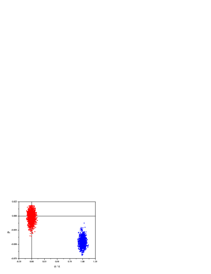
Figure 4: Distribution of confined electrons over the longitudinal phase plane in a system with cubic nonlinearity at $\mu\geq\mu_{c}$; left bunch corresponds to the “linear” case, right – to the “nonlinear” (additional) one

From the figure it follows that the electrons can be confined within not only the “linear” area (minimum of Hamilton function (12)), but the “nonlinear” as well. (The nonlinear stable region disappears in a linear lattice.) RMS sizes and the center of weight positions perfectly correspond to the analytical estimations presented above.

IV Summary. Conclusion

Results of the study on dynamics of synchrotron motion of particles in the storage rings with the nonlinear momentum compaction factor presented in the paper, can be digested as follows:

• Grounded on a simplified model of the storage ring, the finite-difference equations were derived. Hamiltonian treatment of the phase space structure was performed. As was shown, the structure of the phase space is governed by ratios of the ring parameters. An analytical expression for the factor $\mu$, which determines the topology of the longitudinal phase space, was derived.

• Dependencies of the sizes of the equilibrium areas of the synchrotron motion in a nonlinear lattice were derived. Analysis of dependence of the longitudinal acceptance upon the amplitude of rf voltage, and the linear compaction factor at the fixed quadratic nonlinear term was presented. As was shown, the acceptance is growing up only to a definite magnitude which determines by the critical value of parameter $\mu=\mu_{c}$. It was emphasized that in order to maximize the acceptance of a lattice with a small linear momentum compaction factor and a wide energy spread of electrons in the bunches, the system parameters should be chosen close to the critical value of $\mu$.

• To validate the use of smoothed equations of motion, a simulating code was developed. The code is based on the finite-difference equations. The results of simulation manifest a good agreement with the theoretical predictions on the sizes and position of equilibrium areas.

The results obtained allow to make the following conclusion: Enlargement of the energy acceptance of a ring by decreasing of the momentum compaction factor is limited with the nonlinearity in the compaction factor. Decreasing of the linear compaction factor below the certain limit causes the reversed effect — decreasing of the acceptance.

Similar consequence corresponds to the build–up of the rf voltage: Increase of the voltage above a certain limit causes narrowing of possible bunch lengthes while the energy acceptance remains constant. This effect can lead to decrease in the injection efficiency for high rf voltages.

References

- Huang and Ruth (1998) Z. Huang and R. D. Ruth, Phys. Rev. Lett. 80, 976 (1998).
- Loewen (2003) R. J. Loewen, Ph.D. thesis, Stanford (2003).
- Bulyak (2004) E. Bulyak, in Proc. EPAC–2004 (Luzern, Switzerland) (2004), http://accelconf.web.cern.ch/accelconf/ e04/ papers/thpkf063.pdf.
- Crooker et al. (2005) P. P. Crooker, J. Blau, and W. B. Colson, Phys. Rev. ST Accel. Beams 8, 040703 (2005).
- Pellegrini and Robin (1991) C. Pellegrini and D. Robin, Nucl. Instrum. Methods A 301, 27 (1991).
- Lin and da Silva (1993) L. Lin and E. G. da Silva, Nucl. Instrum. Methods A 329, 9 (1993).
- Feikes et al. (2004) J. Feikes, K. Holldack, P. Kuske, G. Wüstefeld, and H.-W. Hübers, ICFA Beam Dynamics Newsletter 35, 82 (2004).