Ground Control to Niels Bohr: Exploring Outer Space with Atomic Physics

To the Sun and Back

8 August 2001 was an exciting day for scientists studying nonlinear dynamics. With a trajectory designed using techniques from the theory of dynamical systems, NASA launched the spacecraft Genesis towards the Sun to collect pieces of it (called solar wind). When Genesis completes its mission (see Fig. 1), scientists may determine not only the composition of the Sun but also whether Earth and the other planets have the same constituents. The samples collected by the Genesis mission of NASA’s Discovery program will be studied extensively for many years now that the spacecraft has returned some of its souvenirs to Earth. A sample return capsule, containing the first extraterrestrial matter returned by a U.S. spacecraft since 1972, was released by Genesis on 8 September 2004 and arrived at the Johnson Space Center in Houston, TX on 4 October. It was subsequently announced in March 2005 that ions of Solar origin were indeed present in one of the wafer fragments [9, 13].

M. Lo of the Jet Propulsion Laboratory, who led the development of the Genesis mission design, worked with Caltech mathematician J. Marsden, Georgia Tech physicist T. Uzer, and West Virginia University chemist C. Jaffé on the statistical analysis of transport phenomena. Why? The Genesis trajectory constitutes a highly unstable orbit (controlled by the Lagrange equilibrium points) of the infamous celestial three body problem studied by H. Poincaré and others. Some of the most dangerous near-earth asteroids and comets follow similar chaotic paths, which have the notorious property that they can be resolved with numerical simulations only up to some finite time.

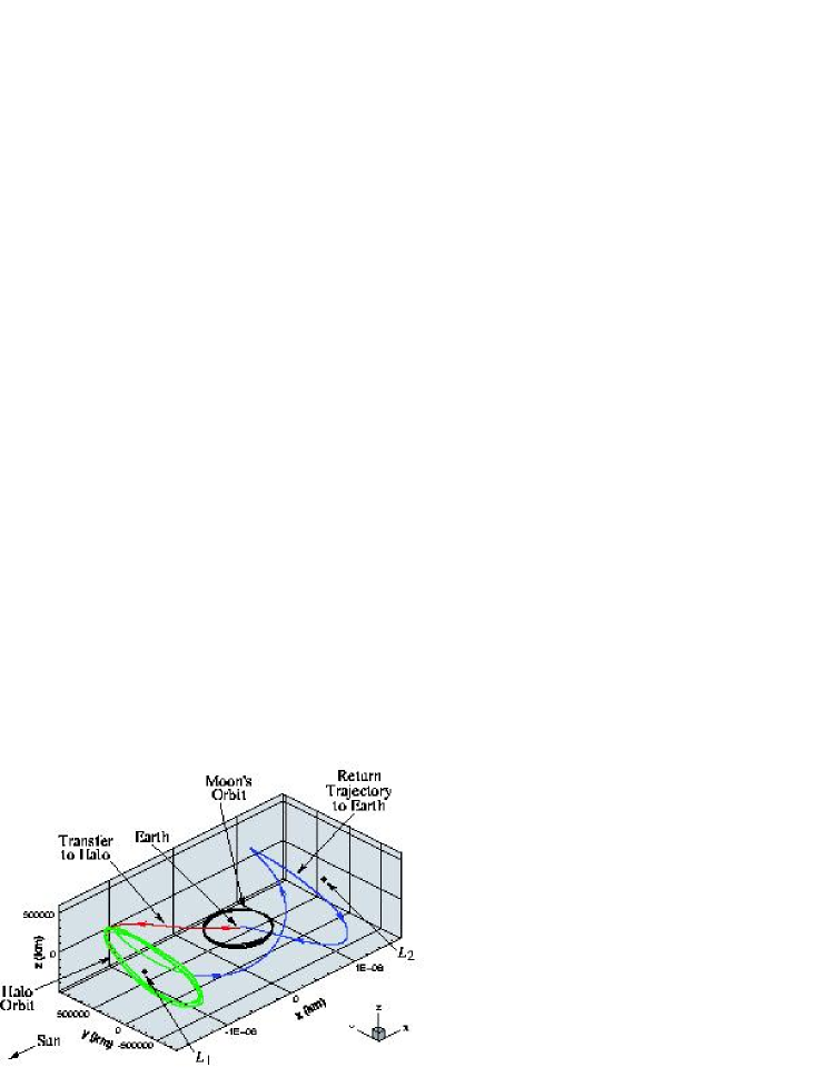
Figure 1: Planned trajectory for the Genesis spacecraft, whose several-year mission is to collect charged particles from the solar wind and return them to Earth. The trajectory was chosen to take Genesis sufficiently far away from Earth’s geomagnetic field so that solar wind samples could be collected before interacting with that field. It reached the first Lagrange point ($L_{1}$) on 16 November 2001, setting up five halo loops about $L_{1}$ (lasting 30 months) that began the scientific portion of the mission. Sample collection lasted from 3 December 2001 until 1 April 2004. Genesis released its sample return capsule on 8 September 2004 (which arrived on 4 October) and then headed back to $L_{1}$, which it was scheduled to leave in February 2005, after which it was slated to begin orbiting around the Sun just inside Earth’s orbit. (Figure courtesy Roby Wilson, Jet Propulsion Laboratory/California Institute of Technology.)

In a turn of events that would have astonished anyone but N. Bohr, we now know that chaotic trajectories identical to those that govern the motions of comets, asteroids, and spacecraft are traversed on the atomic scale by highly excited Rydberg electrons [6, 7, 8, 22, 18]. This almost perfect parallel between the governing equations of atomic physics and celestial mechanics implies that the transport mechanism for these two situations is virtually identical: On the celestial scale, transport takes a spacecraft from one Lagrange point to another until it reaches its desired destination. On the atomic scale, the same type of trajectory transports an electron initially trapped near the atom across an escape threshold (in chemical parlance, across a “transition state”), never to return. The orbits used to design space missions thus also determine the ionization rates of atoms and chemical-reaction rates of molecules!

Recent work [18, 19, 20] also offers hope that researchers may eventually overcome one of the current outstanding challenges of nonlinear science: how does one describe chaotic dynamics in systems with many degrees-of-freedom but still too few to be amenable to the methods of statistical physics? The concept of “chaos” is well-understood only for low-dimensional systems, as few methods deal successfully with higher-dimensional dynamics. Transition state theory is one such tool.

The large-scale chaos present in the Solar System is weak enough that the motion of most planets appears regular on human time scales. Nevertheless, small celestial bodies such as asteroids, comets, and spacecraft can behave in a strongly chaotic manner, and it is important to be able to predict the behavior of populations of these smaller celestial bodies not only to design gravitationally-assisted transport of spacecraft but also to develop a statistical description of populations of comets, near-Earth asteroids, and zodiacal and circumplanetary dust [8].

This is precisely the challenge faced by atomic physicists and chemists in computing ionization rates of atoms and molecules. In brute force approaches, this is accomplished via large numerical simulations that track the orbits of myriad test particles with as many interactions as desired. In practice, however, such techniques are computationally intensive and convey little insight into a system’s key dynamical mechanisms. A theoretically grounded approach relies on transition state theory [8]. “Transition states” are surfaces (manifolds) in the many-dimensional phase space (the set of all possible positions and momenta that particles can attain) that regulate mass transport through bottlenecks in that phase space; the transition rates are then computed using a statistical approach developed in chemical dynamics [18]. In such analyses, one assumes that the rate of intramolecular energy redistribution is fast relative to the reaction rate, which can then be expressed as the ratio of the flux across the transition state divided by the total volume of phase space associated with the reactants.

In the next few sections, we’ll delve a bit deeper into this story. We start with an introduction to transition state theory and then show how this theory from atomic and molecular physics can be used on the much grander celestial scale. We then close with some recent extensions and a brief summary.

Back in the Saddle Again

Before heading off into outer space, we need to examine things on a much smaller scale—namely, simple chemical reactions between ions and small molecules.

Transition state theory has its origins in early 20th century studies of the dynamics of chemical reactions. Consider, for example, the collinear reaction between the hydrogen atom $H$ and the hydrogen molecule $H_{2}$ in which one hydrogen atom switches partners. In the 1930s, Eyring and Polanyi [3] studied this chemical reaction, providing the first calculation of the potential energy surface of a reaction. This surface contains a minimum associated to the reactants and another minimum for the products; they are separated by a barrier that needs to be crossed for the chemical reaction to occur. Eyring and Polanyi defined the surface’s “transition state” as the path of steepest ascent from the barrier’s saddle point. Once crossed, this “transition state” could never be recrossed.

The notion of a transition state as a “surface of no return” defined in coordinate space was immediately recognized as fundamentally flawed, as recrossing can arise from dynamical effects due to coupling terms in the kinetic energy. (See Ref. [6] for further historical details.) Pechukas demonstrated that the surface of minimum flux, corresponding to the transition state, must be an unstable periodic orbit whose projection onto coordinate space connects the two branches of the relevant equipotentials [14]. As a result, these surfaces of minimum flux are called “periodic orbit dividing surfaces” or PODS.

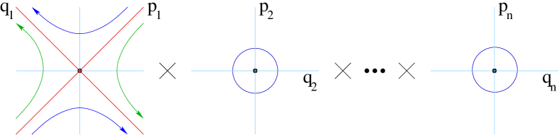
Figure 2: The linearized dynamics of a transition state. One degree-of-freedom yields a pair of real eigenvalues of opposite sign (shown by the saddle projection on the left), and the others give pure imaginary conjugate pairs of eigenvalues (indicated by the center projections) The blue trajectories in the left panel are reactive, whereas the green ones are not.

Despite the specificity of the $H_{2}+H\rightleftharpoons H+H_{2}$ reaction, a transition state is a very general property of Hamiltonian dynamical systems describing how a set of “reactants” evolves into a set of “products” [24]. Transition state theory can be used to study “reaction rates” in a diverse array of physical situations, including atom ionization, cluster rearrangement, conductance through microjunctions, diffusion jumps in solids, and (as we shall discuss) celestial phenomena such as asteroid escape rates [6, 7, 8, 22].

E. Wigner recognized very early that in order to develop a rigorous theory of transition states, one must extend the notions above from configuration space to the phase space of positions and momenta [22, 23]. (Each position-momentum pair constitutes one of the system’s “degrees-of-freedom” [DOF].) The partitioning of phase space into separate regions corresponding to reactants and products thereby becomes the theory’s goal, progress towards which has required advances in both dynamical systems theory and computational hardware.

For two DOF Hamiltonian systems, the stable and unstable manifolds of the orbit discussed provide an invariant partition of the system’s energy shell into reactive and nonreactive dynamics. The defining periodic orbit also bounds a surface in the energy shell (at which the Hamiltonian is constant), partitioning it into reactant and product regions. This, then, defines a surface of no return and yields an unambiguous measure of the flux between reactants and products. In systems with three or more DOF, however, periodic orbits and their associated stable and unstable manifolds do not partition energy shells (their dimensionality is insufficient) [11], so one needs to search instead for higher-dimensional analogs of PODS [22].

Consider an $n$ DOF Hamiltonian system with an equilibrium point, the linearization about which has eigenvalues $\pm\lambda$, $\pm i\omega_{j}$, $j\in\{2\,,\dots\,,n\}$ , where $\lambda\,,\omega_{j}\in\mathbb{R}$. That is, we are considering situations in which the stable and unstable manifolds are each one-dimensional. (There exist chemical reactions with higher-dimensional stable and unstable manifolds, but theoretical chemists do not really know how to deal with them yet.) Also assume that the submatrix corresponding to the imaginary eigenvalues is symmetric, so that its complexification is diagonal. One can then show that in the vicinity of the saddle point, the normal form of this Hamiltonian is [5]

$$H =\lambda q_{1}p_{1}+\sum_{i=2}^{n}\frac{\omega_{i}}{2}(p_{i}^{2}+q_{i}^{2})+f_{1}(q_{2},\dots,q_{n},p_{2},\dots,p_{n},I)$$

$$\quad+f_{2}(q_{2},\dots,q_{n},p_{2},\dots,p_{n})\,,$$ (1)

where $(q_{1},\dots,q_{n},p_{1},\dots,p_{n})$ are the canonical coordinates, $I:=q_{1}p_{1}$, and the functions $f_{1}$ and $f_{2}$ are at least third order and account for all the nonlinear terms in Hamilton’s equations. Additionally, $f_{1}(q_{2},\dots,q_{n},p_{2},\dots,p_{n},I)=0$ when $I=0$. Although (1) is constructed locally, it continues to hold as parameters are adjusted until a bifurcation occurs.

The simplest example is the linear dynamical system with Hamiltonian

$$H=\frac{1}{2}p_{\xi}^{2}-\frac{\kappa^{2}}{2}\xi^{2}+\frac{1}{2}\sum_{i=2}^{n}(p_{i}^{2}+\omega_{i}^{2}q_{i}^{2})$$ (2)

consisting of $n-1$ decoupled linear (“harmonic”) oscillators and a decoupled saddle point, which can be obtained from the linearization of (1) by a rotation in phase space (see Fig. 2). The first DOF $(\xi,p_{\xi})$ gives the “reaction coordinates” and the other $n-1$ DOF are “bath coordinates.” A trajectory is called “reacting” if $\xi$ changes sign as one traverses it.

Such considerations can be generalized from this linear situation to the fully nonlinear Hamiltonian (1) needed to describe chemical reactions by considering higher-dimensional analogs of saddle points called normally hyperbolic invariant manifolds (NHIMs) [22, 21]. The descriptor ‘normally hyperbolic’ means that in the linearization of (1), the growth and decay rates of the dynamics normal to the NHIM (constituting the “reaction”) dominate the growth and decay rates of the dynamics tangent to the NHIM, which is obtained as follows: The dynamics of (1) are described by the $(2n-1)$-dimensional energy surface $H=\mbox{constant}>0$. If $p_{1}=q_{1}=0$, it follows that $\dot{q}_{1}=\dot{p}_{1}=0$, which yields a $(2n-2)$-dimensional invariant manifold, whose intersection with the energy surface gives the NHIM. The $(q_{1},p_{1})$ coordinates describe the directions normal to the NHIM. Additionally, NHIMs persist under perturbations, so one can transform back from (1) to the original Hamiltonian system derived by physical or chemical considerations. The stable and unstable manifolds of the NHIM are known explicitly and act as impenetrable (invariant) boundaries between reactive and nonreactive trajectories [22].

Before proceeding, let’s consider the example of hydrogen ionization in crossed electric and magnetic fields, as described by the Hamiltonian

$$H(x_{1},x_{2},x_{3},P_{1},P_{2},P_{3}) =\frac{1}{2}(P_{1}^{2}+P_{2}^{2}+P_{3}^{2})-\frac{1}{R}$$

$$\quad+\left[\frac{1}{2}(x_{1}P_{2}-x_{2}P_{1})+\frac{1}{8}(x_{1}^{2}+x_{2}^{2})-\epsilon x_{1}-\sqrt{\epsilon}\right]\,,$$ (3)

where $R=\sqrt{(x_{1}+\sqrt{\epsilon})^{2}+x_{2}^{2}+x_{3}^{3}}$. The equilibrium at the origin has two imaginary pairs of eigenvalues and one real pair, so it’s a center-saddle-center. The Hamiltonian (3) can be transformed to its normal form, whose lowest order term is

$$H_{2}=\mu x_{1}P_{1}+\frac{\omega_{1}}{2}(x_{2}^{2}+P_{2}^{2})+\frac{\omega_{2}}{2}(x_{3}^{2}+P_{3}^{2})\,.$$ (4)

As required, the saddle variables $(x_{1},P_{1})$ appear only in the combination $x_{1}P_{1}$, so a NHIM can be constructed as discussed above and one can easily study which trajectories react and which do not.

Hitchhiking the Solar System with Bohr and Poincaré

Volume 7 (1885-86) of Acta Mathematica included the announcement that King Oscar II of Sweden and Norway would award a medal and 2500 kroner prize to the first person to obtain a global general solution to the $n$-body celestial problem [2]. Henri Poincaré, then thirty-one years old, had long been fascinated with celestial mechanics. His first paper, published in 1883, treated some special solutions of the 3-body problem. The following year, Poincaré published a second paper on the topic, but he had not touched celestial mechanics since then. Nevertheless, he had developed new qualitative techniques for studying differential equations that he felt would provide a good intuitive basis for his attempt to solve the $n$-body problem.

In the treatise that resulted from his attempt to win King Oscar II’s prize [15, 16, 17], Poincaré laid the foundations for dynamical systems theory, developing integral invariants to prove his recurrence theorem, a new approach to periodic solutions and stability, and much more. Some of his results clashed with his prior intuition, and there were others that he felt were true but that he was unable to establish rigorously (the world would have to wait for the likes of G. Birkhoff, S. Smale, and others). After more than two years of working on the $n$-body problem, the solution began to take shape. One of the problem’s secrets was revealed by the 3-body problem: Poincaré proved that there did not exist uniform first integrals other than $H=\mbox{constant}$, so that even the 3-body problem could not be “integrated.” Chaos was here to stay!

Now that we have discussed the mathematics of transition states, let’s see how they can help us not only on atomic problems but also on celestial ones. To do this, we will use the old adage that the same equations have the same solutions: Namely, a suitable coordinate change transforms the Hamiltonian describing the celestial restricted three body problem (RTBP) into the Hamiltonian (3) describing hydrogen ionization in crossed electric and magnetic fields [8]. The term “restricted” is used when the mass of one body is assumed to be so small that it does not influence the motion of the other two bodies, which follow circular orbits around their center of mass. It is also assumed that all three orbits lie in a common plane [2, 10].

In conventional coordinates, the RTBP is described by the Hamiltonian

$$H=\frac{1}{2}(p_{x}^{2}+p_{y}^{2})-(xp_{y}-yp_{x})-\frac{1-\mu}{r_{1}}-\frac{\mu}{r_{2}}-\frac{1}{2}\mu(1-\mu)=E\,,$$ (5)

where $E$ is the energy, $r_{1}=\sqrt{(x+\mu)^{2}+y^{2}}$, $r_{2}=\sqrt{(x-1+\mu)^{2}+y^{2}}$, and the masses of the bodies are $m_{s}=1-\mu$ and $m_{p}=\mu<m_{s}$. (The notation is chosen so that one thinks of $m_{s}$ as the Sun’s mass and $m_{p}$ as a planet’s mass.) The coordinate system rotates with the period of Jupiter about the Sun-Jupiter center of mass. The Sun and Jupiter are located respectively, at $(-\mu,0)$ and $(1-\mu,0)$. The position of the the third body (say, an asteroid) relative to the Sun and the planet is $(x,y)$.

An example is provided by Jupiter’s comets such as Oterma which shuttle back and forth between complex heliocentric orbits lying, respectively, interior and exterior to Jupiter’s orbit [8] (see Fig. 3). (Oterma lies in the same energy regime as Shumaker-Levy 9, so it is destined to one day crash into Jupiter.) Jupiter often temporarily ‘captures’ such comets while they make these transitions. The interior orbits are generally near a 3:2 resonance, with Oterma making three revolutions about the Sun for every two solar revolutions of Jupiter (in the inertial frame), whereas the exterior ones are near a 2:3 resonance. In a frame rotating with Jupiter, the transition between resonances occurs in a “bottleneck” region in configuration space.

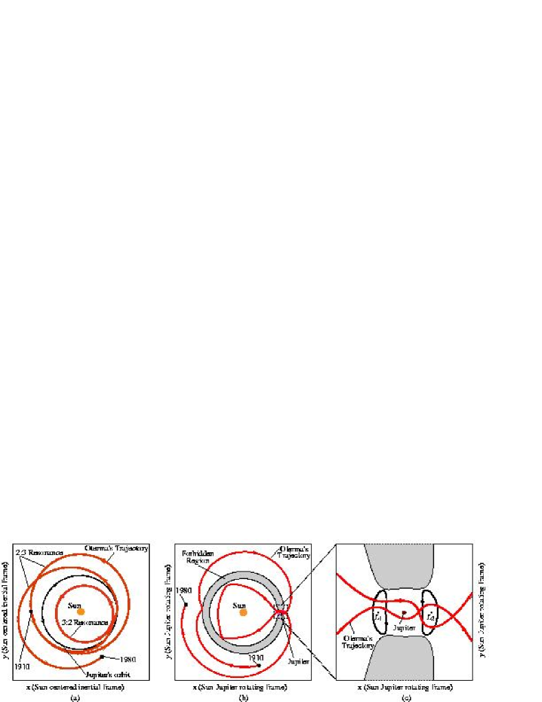
Figure 3: Resonance transition of the Jovian comet Oterma. (a) The dynamics in heliocentric coordinates. (b) The dynamics in a reference frame rotating with Jupiter. (c) Magnified view of the bottleneck region from (b). (Figure courtesy Shane D. Ross, University of Southern California.)

The celebrated “Jacobi integral” (a constant of motion) provides a dynamical invariant that divides phase space into reactant (interior) and product (exterior) regions, which are separated by the narrow bottleneck containing Jupiter and two of the Lagrange points, $L_{1}$ and $L_{2}$. The passage of celestial bodies like comets through the bottleneck is then regulated by phase space structures near $L_{1}$ and $L_{2}$, which are both saddle points. The transition states in this problem, controlling transport through the bottleneck and hence the conversion of “reactants” to “products,” are the periodic orbits around $L_{1}$ and $L_{2}$. With these structures identified, C. Jaffé et al. have accurately computed average transport rates (corresponding to asteroid escape rates) using Rice-Ramsperger-Kassel-Marcus theory and checked the predicted rates against large-scale numerical simulations [8].

Meanwhile, Back on Earth…

The story doesn’t end with the work discussed in this note. On the practical side, discussions at NASA are currently underway about the possibility of an extended Genesis mission that would keep the spacecraft in the Earth-Moon system for the next several years [9].

On the theoretical side, the mathematics, physics, and chemistry communities remain hard at work. Recent discoveries include a computational procedure based on NHIMs to detect high-dimensional chaotic saddles in three DOF Hamiltonian systems (and the application of this technology to, for example, the three-dimensional Hill’s problem) [19], mathematical refinements of earlier constructions of transition states [20], and the effect of noise on transition states [1]. Current work on space mission design includes the use of set-oriented methods and ideas from graph theory to go beyond transition state theory [12] and the merging of tube dynamics with a Monte Carlo approach to examine the invariant manifolds emanating from transition states [4].

It is a time-honored scientific tradition that the same equations have the same solutions. When it comes to $3$-body problems, this implies that the same chaotic trajectories that govern the motions of comets, asteroids, and spacecraft are traversed on the atomic scale by highly excited Rydberg electrons. Such unanticipated connections between microscopic and celestial phenomena are not only intellectually gratifying but also have practical engineering applications in the aerospace and chemical industries. Moreover, the progress made would hardly be conceivable without this particular mix of specialists recruited by M. Lo. Clearly, chemists, astronomers, and mathematicians have much to discuss!

Additionally, while it is paramount in many problems to slay the dragon of chaos so that order can reign, just the opposite is true here—the goal is to create a big enough (chaotic) saddle and ride this dragon on the (Normally Hyperbolic) Invariant Manifold Superhighway! The Genesis mission shows that chaos can, in fact, be good.

References

- [1] T. Bartsch, R. Hernandez, and T. Uzer, The transition state in a noisy environment. Submitted, February 2005.
- [2] F. Diacu and P. Holmes, Celestial Encounters: The Origins of Chaos and Stability, Princeton University Press, Princeton, NJ, 1996.
- [3] H. Eyring and M. Polanyi, On simple gas reaction, Zeitschrift für physikalische Chemie B, 12 (1931), pp. 279–311.
- [4] F. Grabern, W. S. Koon, J. E. Marsden, and S. D. Ross, Theory and computation of non-RRKM lifetime distributions and rates in chemical systems with three or more degrees of freedom. Submitted, February 2005.
- [5] J. Guckenheimer and P. Holmes, Nonlinear Oscillations, Dynamical Systems, and Bifurcations of Vector Fields, No. 42 in Applied Mathematical Sciences, Springer-Verlag, New York, NY, 1983.
- [6] C. Jaffé, D. Farrelly, and T. Uzer, Transition state in atomic physics, Physical Review A, 60 (1999), pp. 3833–3850.
- [7] C. Jaffé, D. Farrelly, and T. Uzer, Transition state theory without time-reversal symmetry: Chaotic ionization of the hydrogen atom, Physical Review Letters, 84 (2000), pp. 610–613.
- [8] C. Jaffé, S. D. Ross, M. W. Lo, J. Marsden, D. Farrelly, and T. Uzer, Statistical theory of asteroid escape rates, Physical Review Letters, 89 (2002), No. 011101.
- [9] Jet Propulsion Laboratory, Genesis: Search for origins. genesismission.jpl.nasa.gov, April 15, 2005.
- [10] W. S. Koon, M. W. Lo, J. E. Marsden, and S. D. Ross, Heteroclinic connections between periodic orbits and resonance transitions in celestial mechanics, Chaos, 10 (2000), pp. 427–469.
- [11] A. J. Lichtenberg and M. A. Lieberman, Regular and Chaotic Dynamics, No. 38 in Applied Mathematical Sciences, Springer-Verlag, New York, NY, 2nd ed., 1992.
- [12] J. E. Marsden and S. D. Ross, New methods in celestial mechanics and mission design. In preparation, May 2005.
- [13] National Aeronautics and Space Administration, Genesis and the search for origins. www.nasa.gov/mission_pages/genesis/main, April 15, 2005.
- [14] P. Pechukas, Dynamics of Molecular Collisions, Plenum, New York, NY, 1976, ch. 6, Part B.
- [15] H. Poincaré, New Methods of Celestial Mechanics, Volume I: Periodic Solutions, The Non-existence of Integral Invariants, Asymptotic Solutions, Dover Publications, New York, NY, 1957.
- [16] , New Methods of Celestial Mechanics, Volume II: Methods of Newcomb, Gylden, Lindstedt, and Bohlin, Dover Publications, New York, NY, 1957.
- [17] , New Methods of Celestial Mechanics, Volume III: Integral Invariants, Periodic Solutions of the Second Type, Doubly Asymptotic Solutions, Dover Publications, New York, NY, 1957.
- [18] T. Uzer, C. Jaffé, J. Palacián, P. Yanguas, and S. Wiggins, The geometry of reaction dynamics, Nonlinearity, 15 (2002), pp. 957–992.
- [19] H. Waalkens, A. Burbanks, and S. Wiggins, A computational procedure to detect a new type of high-dimensional chaotic saddle and its application to the 3D Hill’s problem, Journal of Physics A: Mathematical and General, 37 (2004), pp. L257–L265.
- [20] H. Waalkens and S. Wiggins, Direct construction of a dividing surface of minimal flux for multi-degree-of-freedom systems that cannot be recrossed, Journal of Physics A: Mathematical and General, 37 (2004), pp. L435–L445.
- [21] S. Wiggins, Normally Hyperbolic Invariant Manifolds in Dynamical Systems, Springer-Verlag, New York, NY, 1994.
- [22] S. Wiggins, L. Wiesenfeld, C. Jaffé, and T. Uzer, Impenetrable barriers in phase space, Physical Review Letters, 86 (2001), pp. 5478–5481.
- [23] E. Wigner, Calculation of the rate of elementary association reactions, Journal of Chemical Physics, 5 (1937), pp. 720–725.
- [24] , The transition state method, Transactions of the Faraday Society, 34 (1938), pp. 29–41.