Dynamics and thermodynamics of axisymmetric flows:
I. Theory

Abstract

We develop new variational principles to study the structure and the stability of equilibrium states of axisymmetric flows. We show that the axisymmetric Euler equations for inviscid flows admit an infinite number of steady state solutions. We find their general form and provide analytical solutions in some special cases. The system can be trapped in one of these steady states as a result of an inviscid violent relaxation. We show that the stable steady states maximize a (non-universal) $H$-function while conserving energy, helicity, circulation and angular momentum (robust constraints). This can be viewed as a form of generalized selective decay principle. We derive relaxation equations which can be used as numerical algorithm to construct nonlinearly dynamically stable stationary solutions of axisymmetric flows. We also develop a thermodynamical approach to predict the equilibrium state at some fixed coarse-grained scale. We show that the resulting distribution can be divided in two parts: one universal coming from the conservation of robust invariants and one non-universal determined by the initial conditions through the fragile invariants (for freely evolving systems) or by a prior distribution encoding non-ideal effects such as viscosity, small-scale forcing and dissipation (for forced systems). Finally, we derive a parameterization of inviscid mixing to describe the dynamics of the system at the coarse-grained scale. A conceptual interest of this axisymmetric model is to be intermediate between 2D and 3D turbulence.

I Introduction

The ubiquity of rotating systems in astrophysics and geophysics makes axisymmetric flows a classical paradigm. In the laboratory, two axisymmetric devices, the Taylor-Couette flow and the von Kármán flow, have become a standard to investigate issues such as super-critical and sub-critical stability Prigent et al. (2002), fluctuation of global quantities Aumaître et al. (2001); Labbé et al. (1996) or turbulent transport Taylor (1923); Lathrop et al. (1992); Marié and Daviaud (2004). However, many basic issues regarding stability and turbulence in axisymmetric flows still remain unsolved. For example, one still fails to understand the onset of turbulence or the equilibrium state in Taylor-Couette with outer rotating cylinder Dubrulle et al. (2005), or the recent bifurcation of the turbulent state observed in von Kármán flow Ravelet et al. (2004).

In the past, dynamical stability and equilibrium properties of flows have often been studied using variational Chandrasekhar (1961) or maximization Busse (1996) principles. Examples of application to axisymmetric flows include necessary criteria for instability or turbulent velocity profiles in Taylor-Couette flow. Maximization or minimization principles have also been used to give sufficient criteria of nonlinear dynamical stability Holm et al. (1985). One interest of these methods is their robustness, in the sense that they mostly depend on characteristic global quantities of the system (such as the energy) but not necessarily on small-scale dissipation or boundary conditions. More recently, optimization methods have been developed within the framework of statistical mechanics for two-dimensional (2D) perfect fluids. In that case, variational principles based on entropy maximization determine conditions of thermodynamical stability. Onsager Onsager (1949) first used a Hamiltonian model of point vortices and identified turbulence as a state of negative temperature leading to the coalescence of vortices of same sign Montgomery and Joyce (1974). Further improvements were provided by Kuzmin Kuzmin (1982), Miller Miller (1990) and Robert and Sommeria Robert and Sommeria (1991) who independently introduced a discretization of the vorticity in a certain number of levels to account for the continuous nature of vorticity. Using the maximum entropy formalism of statistical mechanics Jaynes (1957), it is then possible to obtain the shape of the metaequilibrium solution of Euler’s equation as well as the distribution of the fine-grained fluctuations around it. A variety of solutions are found and the bifurcation diagram displays a rich structure as illustrated by Chavanis & Sommeria Chavanis and Sommeria (1996) in a particular limit of the statistical theory. Two-dimensional turbulence is however very peculiar since it misses vortex stretching, one essential ingredient in 3D turbulence. The adaptation of these methods to more realistic situations is therefore not obvious.

In the case where the system admits a scalar invariant ($D_{t}\sigma=\partial_{t}\sigma+{\bf u}\cdot{\bf\nabla}\sigma=0$), one can show that a Liouville theorem holds (incompressibility of the motion in phase space). Indeed, the proof given by Kraichnan & Montgomery Kraichnan and Montgomery (1980) in the case of 2D turbulence can be extended to any dimensional turbulence with a conserved quantity. This is in fact the case for axisymmetric flows where the symmetry imposes angular momentum conservation. Due to violent relaxation, the system is expected to reach a metaequilibrium state which is a steady solution of the axisymmetric Euler equations. The purpose of the present paper is to derive explicit results regarding nonlinear dynamical stability and thermodynamical equilibrium properties of axisymmetric flows using optimization methods.

In the first part of the paper (Sec. II), we consider the nonlinear dynamical stability of stationary solutions of the axisymmetric Euler equations (i.e. without viscosity). These equations are written in Sec. II.1 and the general form of stationary solutions is obtained in Sec. II.2. In Sec. II.3, we list the conservation laws of the axisymmetric Euler equations. We find non trivial invariants in addition to the usual ones. In Sec. II.4, we show that the equilibrium solutions can be obtained by extremizing a functional built with all the invariants. The fact that this optimization procedure returns the general stationary solution means that we have found all the invariants. In Sec. II.5, we distinguish between fragile (Casimirs) and robust (energy, helicity, circulation, angular momentum…) invariants. We argue that, in the presence of viscosity or coarse-graining, the metaequilibrium state maximizes a certain (non-universal) H-function while conserving the robust constraints. This is similar to the case of pure 2D hydrodynamics Chavanis (2003, 2005, 2005, 2006) except for the replacement of vorticity by angular momentum. In Sec. II.6, we propose a numerical algorithm based on the maximization of the production of an H-function while conserving the robust constraints. This can be used to compute numerically arbitrary nonlinearly dynamically stable stationary solutions of the axisymmetric Euler equations. This is similar to the relaxation equations proposed by Chavanis Chavanis (2003, 2005, 2005) in pure 2D hydrodynamics. In Sec. II.7, we provide simple analytical steady solutions of axisymmetric equilibrium flows. In the second part of the paper (Sec. III), we develop the statistical mechanics of such flows to predict the metaequilibrium state. The statistical equilibrium state is obtained by maximizing a mixing entropy (Sec. III.1) while taking into account all the constraints of the dynamics. This yields a Gibbs state (Sec. III.2) which gives the equilibrium coarse-grained angular momentum as well as the fluctuations around it. We check that the coarse-grained field is a stationary solution of the axisymmetric Euler equations. However, since the Casimirs are not conserved on the coarse-grained scale, the distribution of fluctuations is non universal and depends on the initial conditions (or fine-grained constraints). This is also the case for the coarse-grained field. In Sec. III.4, we use a maximization of the entropy production to derive relaxation equations towards the statistical equilibrium state. This is similar to the approach proposed by Robert & Sommeria Robert and Sommeria (1992) in pure 2D hydrodynamics. Finally, in Sec. III.5, we introduce the notion of prior distribution of fluctuations for systems that are forced at small scales. We show that the coarse-grained field maximizes at statistical equilibrium a generalized entropy fixed by the prior distribution. Thus, the relaxation equations based on the maximization of the production of generalized entropy (Sec. II.6) can also provide a parameterization of axisymmetric turbulence in the presence of a small-scale forcing Chavanis (2003, 2005, 2005).

II Dynamical stability of axisymmetric flows

II.1 The axisymmetric Euler equations

The Euler equations describing the dynamics of an inviscid incompressible axisymmetric flow can be written in cylindrical coordinates $(r,\theta,z)$ as:

$$\frac{1}{r}\partial_{r}(ru)+\partial_{z}w = 0\;,$$ (1)

$$\partial_{t}u+u\partial_{r}u+w\partial_{z}u-\frac{v^{2}}{r} = -\frac{1}{\rho}\partial_{r}p\;,$$

$$\partial_{t}v+u\partial_{r}v+w\partial_{z}v+\frac{vu}{r} = 0\;,$$

$$\partial_{t}w+u\partial_{r}w+w\partial_{z}w = -\frac{1}{\rho}\partial_{z}p\;,$$

where $(u,v,w)$ denote the components of the velocity in a cylindrical referential. Note that the third equation expresses the conservation of the angular momentum $\sigma=rv$. The two other equations for $u$ and $w$ involve a pressure field determined through incompressibility. However, it can be eliminated by using the stream-function vorticity formulation Lopez (1990). The two new scalar variables are the azimuthal component of the vorticity $\omega_{\theta}=\partial_{z}u-\partial_{r}w$ and the stream function $\psi$ defined by:

$$u=-\frac{1}{r}\partial_{z}\psi,\qquad\text{and}\qquad w=\frac{1}{r}\partial_{r}\psi\;.$$

The existence of a stream function results from the incompressibility and the axisymmetry of the flow. In this formulation, the system (1) can be rewritten:

$$\partial_{t}v-\frac{1}{r}\partial_{z}\psi\partial_{r}v+\frac{1}{r}\partial_{r}\psi\partial_{z}v-\frac{1}{r^{2}}\partial_{z}\psi v = 0\;,$$ (2)

$$\partial_{t}\omega_{\theta}-\frac{1}{r}\partial_{z}\psi\partial_{r}\omega_{\theta}+\frac{1}{r}\partial_{r}\psi\partial_{z}\omega_{\theta}+\partial_{z}\psi\frac{\omega_{\theta}}{r^{2}} = \partial_{z}\left(\frac{v^{2}}{r}\right)\;.$$

By definition, the azimuthal component of the vorticity is related to the stream function by:

$$\partial_{r}\left(\frac{1}{r}\partial_{r}\psi\right)+\frac{1}{r}\partial^{2}_{z}\psi=-\omega_{\theta}\;.$$ (3)

We now introduce two new fields, the angular momentum $\sigma=rv$ and $\xi$ which is related to the azimuthal component of the vorticity by $\xi=\omega_{\theta}/r$. Changing variables from $(r,z)$ to $(y,z)$ where $y=r^{2}/2$, we can finally recast the equations (2) and (3) as

$$\partial_{t}\sigma+\{\psi,\sigma\} = 0\;,$$ (4)

$$\partial_{t}\xi+\{\psi,\xi\} = \partial_{z}\left(\frac{\sigma^{2}}{4y^{2}}\right)\;,$$

$$\Delta_{*}\psi\equiv\frac{1}{2y}\partial^{2}_{z}\psi+\partial^{2}_{y}\psi = -\xi\;,$$

where $\{\psi,\phi\}=\partial_{y}\psi\partial_{z}\phi-\partial_{z}\psi\partial_{y}\phi$ is the Jacobian and $\Delta_{*}$ is a pseudo-Laplacian. We also note that $u_{z}=\partial_{y}\psi=w$ and $u_{y}=-\partial_{z}\psi=ru$. This formulation of the axisymmetric Navier-Stokes equation has to be supplemented by appropriate boundary conditions. For reasons which will become clear later, we delay this topic until the discussion of the conservation laws (section II.3 and Appendix A). In the following, we study axisymmetric equilibrium flows by using the system of equations (4) instead of (1). We look for stationary solutions and investigate their stability by using variational methods. Notice that only two scalar variables are sufficient to prescribe such flows: we use $\sigma$, related to the azimuthal component of the velocity field and $\xi$, related to the azimuthal component of the vorticity.

II.2 Stationary solutions

We now derive the general form of stationary solutions of the axisymmetric Euler equations (4). Noting that

$$\{\frac{\sigma}{2y},\sigma\}=-\partial_{z}\left(\frac{\sigma^{2}}{4y^{2}}\right)\;,$$ (5)

the stationary equations can be written

$$\{\psi,\sigma\}=0\qquad\text{and}\qquad\{\psi,\xi\}+\{\frac{\sigma}{2y},\sigma\}=0.$$ (6)

The first equation is satisfied if

$$\psi=R(\sigma),$$ (7)

where $R$ is an arbitrary function. Using the general identity

$$\{R(\sigma),\xi\}=R^{\prime}(\sigma)\{\sigma,\xi\}=\{\sigma,\xi R^{\prime}(\sigma)\},$$ (8)

the second equation becomes

$$\{\sigma,\xi R^{\prime}(\sigma)\}+\{\frac{\sigma}{2y},\sigma\}=0,$$ (9)

or, equivalently

$$\{\sigma,\xi R^{\prime}(\sigma)-\frac{\sigma}{2y}\}=0.$$ (10)

Therefore, the general stationary solution of Eqs. (4) is of the form

$$\psi=R(\sigma)\quad\text{and}\quad\xi R^{\prime}(\sigma)-\frac{\sigma}{2y}=G(\sigma),$$ (11)

where $R$ and $G$ are arbitrary functions. If $R$ is monotonic, we can set $f=R^{-1}$ and we get $\sigma=f(\psi)$ and

$$\xi-\frac{f(\psi)}{2y}\frac{1}{R^{\prime}[R^{-1}(\psi)]}=g(\psi).$$ (12)

Using the identity

$$\frac{1}{R^{\prime}[R^{-1}(\psi)]}=f^{\prime}(\psi),$$ (13)

we finally obtain

$$\sigma=f(\psi),$$

$$-\Delta_{*}\psi=\xi=\frac{f(\psi)}{2y}f^{\prime}(\psi)+g(\psi),$$ (14)

where $f$ and $g$ are arbitrary functions. We can obtain these equations directly if we note that Eq. (6-a) is satisfied if $\sigma=f(\psi)$. Then, using the general identity

$$\biggl{\{}\frac{\sigma}{2y},f(\psi)\biggr{\}}=\biggl{\{}\frac{f^{\prime}(\psi)\sigma}{2y},\psi\biggr{\}},$$ (15)

we can rewrite Eq. (6-b) in the form

$$\biggl{\{}\psi,\xi-\frac{f(\psi)f^{\prime}(\psi)}{2y}\biggr{\}}=0,$$ (16)

which leads to Eq. (14-b). Equation (14-b) is the fundamental differential equation of the problem which must be supplemented by appropriate boundary conditions. Some particular solutions of this equation will be given in Sec. II.7. We will first show that the stationary solutions can be found by a variational principle depending only on the conservation laws of the system.

II.3 Conservation laws

Axisymmetric inviscid flows satisfy a number of conservation laws. We here give the expression of these conserved quantities and postpone corresponding proofs in Appendix A. To derive the two first conservation laws, we must assume that the function $\psi$ vanishes on the boundary of the domain which amounts to considering that the normal component of the velocity is zero at the boundary. This condition is not sufficient for deriving the third conservation law and one must also suppose that either $\sigma$ or $\xi$ vanishes at the boundary.

• The first conserved quantity is the total energy

  $$E = \frac{1}{2}\int(u^{2}+w^{2})\,rdrdz+\frac{1}{2}\int v^{2}\,rdrdz$$

  $$= \frac{1}{2}\int\xi\psi\,dydz+\frac{1}{4}\int\frac{\sigma^{2}}{y}\,dydz.$$

  Here, we have normalized the energy by $2\pi$ and used integration by parts to obtain the second expression.

• Because of (4-a) any function of the angular momentum is also an invariant noted as

  $$I_{f}=\int f(\sigma)\,dydz\;.$$ (18)

  These functionals are called the Casimirs. The conservation of all the Casimirs is equivalent to the conservation of all the moments of $\sigma$, denoted $I_{n}=\int\sigma^{n}\,dydz$. The first moment is the total angular momentum $I=\int\sigma\,dydz$.
  If $\sigma=0$ or, more generally, $\sigma=\sigma(y)$, then $\xi$ is conserved via (4-b). In that case, $\xi$ is called a potential vorticity (or a pseudo-vorticity) and there is an additional class of Casimir invariants: $I_{h}=\int h(\xi)\,dydz$. We ignore this difficulty linked to a sort of “degeneracy” for the time being. Note that the situation where only the pseudo-vorticity is conserved (i.e the case $\sigma=0$) has been treated in Mohseni (2001). In that case, the generalization essentially amounts to replacing the Laplacian $\Delta$ in pure 2D flows by the pseudo-Laplacian $\Delta_{*}$. The situation that we consider here is complicated by the existence of additional invariants such as helicity discussed below. This makes our situation intermediate between pure 2D turbulence and 3D turbulence, an interesting feature of our model.

• Like in any 3D flows, the total helicity, $H=\int{\bf v}\cdot\boldsymbol{\omega}\,rdrdz=\int\sigma\xi\,dydz,\;$ is also an invariant. However, more generally, we show in Appendix A the conservation of a generalized helicity

  $$H_{F}=\int\xi F(\sigma)\,dydz\;,$$ (19)

  where $F$ is an arbitrary function. In particular, the total vorticity $H_{0}=\Gamma=\int\xi\,dydz$ is conserved.
  

II.4 Nonlinear dynamical stability

From the integral constraints discussed previously, we can build a functional ${\cal F}=E+I_{f}+H_{F}$. This functional is an invariant of the inviscid dynamics. This is an extension of the Energy-Casimir functional considered in Holm et al. (1985). It is also similar to a free energy in thermodynamics. We now show that a critical point of ${\cal F}$ determines a stationary solution of the axisymmetric Euler equations. Furthermore, following Holm et al. (1985), a minimum or a maximum of ${\cal F}$ provides a condition of formal nonlinear dynamical stability. This means that a perturbation will remain close (in some norm) to this minimum or maximum. Writing

$$\delta{\cal F}=\delta(E+I_{f}+H_{F})=0,$$ (20)

and taking variations on $\sigma$ and $\xi$, we obtain

$$\psi+F(\sigma)=0\quad\text{and}\quad\frac{\sigma}{2y}+f^{\prime}(\sigma)+\xi F^{\prime}(\sigma)=0\,.$$ (21)

Setting $R=-F$ and $G=f^{\prime}$, we recover the equations (11) characterizing a steady solution of the axisymmetric Euler equations. Since we obtain the general form of steady states it means that we have found all the conservation laws of the axisymmetric Euler equations.

In order to gain some physical insight in the problem, we consider from now on a simpler model where only the usual helicity $H$ and the total vorticity $\Gamma$ are conserved instead of all the generalized helicities. This is similar to our choice of restricting ourselves to the Chandrasekhar model in axisymmetric MHD Leprovost et al. (2005). We define

$$S[\sigma]=-\int C(\sigma)\,dydz\,,$$ (22)

where $C$ is an arbitrary convex function, i.e. $C^{\prime\prime}>0$. Such functionals are exactly conserved by the axisymmetric equations (they are particular Casimirs). Therefore, as in 2D hydrodynamics Ellis et al. (2002), the maximization of $S$ at fixed energy $E$, helicity $H$, circulation $\Gamma$ and angular momentum $I$ determines a nonlinearly dynamically stable stationary solution of the axisymmetric Euler equations. This refined stability criterion is stronger than the maximization of $J=S-\beta E-\mu H-\nu\Gamma-\alpha I$ which just provides a sufficient condition of formal nonlinear dynamical stability Holm et al. (1985). The difference between these two criteria is similar to a notion of ensemble inequivalence in thermodynamics (where $S$ plays the role of an entropy and $J$ the role of a free energy) Chavanis (2003); Bouchet and Barré (2005). We shall not prove the nonlinear dynamical stability result in this paper and refer to Ellis et al. (2002) for a precise discussion in 2D hydrodynamics. In Sec. II.5, we show, however, that this maximization principle is consistent with the phenomenology of axisymmetric turbulence provided that $\sigma$ is interpreted as the coarse-grained angular momentum.

To first order, the variational problem takes the form:

$$\delta S-\beta\delta E-\mu\delta H-\gamma\delta\Gamma-\alpha\delta I=0,$$ (23)

where $\alpha$, $\beta$, $\mu$ and $\gamma$ are appropriate Lagrange multipliers. This variational problem determining nonlinearly dynamically stable stationary solutions of the Euler equations is similar to a variational problem in thermodynamics where $S$ plays the role of an entropy and $\beta$ the role of an inverse temperature Chavanis (2003, 2005). Using the expression of $S$, $E$, $H$, $\Gamma$ and $I$, we find that the solutions of (23) valid for any $\delta\sigma$ and $\delta\xi$ satisfy

$$\beta\psi=-\mu\sigma-{\gamma},$$ (24)

$$-C^{\prime}(\sigma)={\beta}\frac{\sigma}{2y}+\mu\xi+\alpha,$$

which is a particular case of Eq. (11). Thus, the variational principle selects stationary solutions of the axisymmetric Euler equations. We note that when only the ordinary helicity is considered (instead of the general helicity), we obtain a linear relationship between $\sigma$ and $\psi$. This is similar to the linear relationship between velocity ${\bf V}$ and magnetic field ${\bf B}$ in MHD Leprovost et al. (2005). Note that we have just considered the first order variations here. To check if solutions (24) are real maxima of $S$, one has to look for second-order variations as discussed in Appendix B.

II.5 $H$-functions and generalized selective decay principle

We now introduce the notion of fine-grained and coarse-grained fields. The first one refers to the original field defined on all points of space and time and the second one to a smooth version of it, where a local average of the field has been performed. The coarse-grained field is also defined on every point of space but contains less small-scale structure than the original field. Since the functionals (22) calculated with the fine-grained field $\sigma$ are particular Casimirs, they are rigorously conserved by the fine-grained dynamics. In contrast, as Tremaine et al. Tremaine et al. (1986) have shown for the Vlasov equation in stellar dynamics, the functionals of the form (22) calculated with the coarse-grained field increase as mixing proceeds. This is similar to the Boltzmann $H$-theorem in kinetic theory except that the Vlasov equation does not single out a particular functional. This property is true also in the present context since Eq. (4-a) plays the same role as the Vlasov equation. Therefore, $S[\overline{\sigma}]=-\int C(\overline{\sigma})d{\bf r}$ increases along the dynamics in the sense that $S[\overline{\sigma}({\bf r},t)]\geq S[\overline{\sigma}({\bf r},0)]$ for all $C$ and all $t\geq 0$ where it is assumed that, initially, the flow is not mixed: $\overline{\sigma}({\bf r},0)=\sigma({\bf r},0)$ (note that nothing is implied concerning the relative values of $S(t)$ and $S(t^{\prime})$ for $t\geq 0$, $t^{\prime}\geq 0$). Following Tremaine et al. (1986), these functionals will be called $H$-functions (or generalized $H$-functions). They also increase (in that case monotonically) in the presence of viscosity since the equations of motion now become:

$$\partial_{t}\sigma+\{\psi,\sigma\} = \nu r\biggl{(}\Delta\frac{\sigma}{r}-\frac{\sigma}{r^{3}}\biggr{)}=\nu\biggl{[}\Delta\sigma-\frac{2}{r}\frac{\partial\sigma}{\partial r}\biggr{]}\;,$$ (25)

$$\partial_{t}\xi+\{\psi,\xi\} = \partial_{z}\left(\frac{\sigma^{2}}{4y^{2}}\right)+\frac{\nu}{r}\biggl{[}\Delta(r\xi)-\frac{\xi}{r}\biggr{]}=\nu\biggl{[}\Delta\xi+\frac{2}{r}\frac{\partial\xi}{\partial r}\biggr{]}\;,$$

and by integration by part, one can show that $\dot{S}=\nu\int C^{\prime\prime}(\sigma)(\nabla\sigma)^{2}d{\bf r}\geq 0$. By contrast, the integrals $E$, $\Gamma$, $H$, and $I$ are exactly or approximately conserved on the coarse-grained scale (i.e. when they are calculated with the coarse-grained field) or in the presence of a small viscosity. For example, in the presence of viscosity, the kinetic energy evolves such that $\dot{E}=-\nu\int\boldsymbol{\omega}^{2}\,d{\bf r}$. It is easy to show that for axisymmetric fields, the total vorticity $\boldsymbol{\omega}=r\xi{\bf e_{\theta}}+{\bf\nabla}\times(\sigma/r\,{\bf e_{\theta}})$ vanishes in the long time limit. The demonstration is similar to Cowling’s Cowling (1934) theorem of dynamo theory which states that an axisymmetric magnetic field cannot grow in an axisymmetric velocity field: the first equation in (25) shows that $\sigma\rightarrow 0$ for large time and, consequently, the source term in the second equation $\partial_{z}\left(\sigma^{2}/4y^{2}\right)$ vanishes in the long time limit, which implies that $\xi\rightarrow 0$. Thus, for axisymmetric flows, both components of the vorticity vanish in the long time limit and the energy is approximately conserved. In a similar way, it can be shown that $\Gamma$, $H$, and $I$ are approximately conserved and must therefore be strictly taken into account in the constraints. Therefore, the functionals $S$ can be viewed as fragile invariants while the constraints $E$, $\Gamma$, $H$, and $I$ are robust invariants. This generalizes the notion of selective decay in pure 2D turbulence where the enstrophy decays while the energy is approximately conserved. In fact, minus the enstrophy is a particular H-function Chavanis (2003, 2005, 2006). The same discussion applies in the present context. On the basis of this phenomenological principle, we expect that, due to chaotic mixing and violent relaxation, the system will reach a metaequilibrium state which maximizes a certain $H$-function (non-universal) at fixed $E$, $\Gamma$, $H$, and $I$. This phenomenological argument returns the variational principle (23). Since this metaequilibrium state results from turbulent mixing, it is expected to be particularly robust and should possess properties of nonlinear dynamical stability. Therefore, the stability arguments given previously are consistent with the phenomenology of axisymmetric turbulence, provided that $\sigma$ is interpreted as the coarse-grained angular momentum $\overline{\sigma}$. This is remarkable because the two arguments are relatively independent: there is no direct notion of decay (of $-S$) in the first argument while this lies at the heart of the second. In fact, the phenomenology of violent relaxation explains how an inviscid system can reach a nonlinearly dynamically stable stationary state on a coarse-grained scale which is a maximum of a certain $H$-function at fixed robust constraints (while $S[\sigma]$ is rigorously conserved on the fine-grained scale). The point is that during mixing $D\overline{\sigma}/Dt\neq 0$ and the $H$-functions $S[\overline{\sigma}]$ increase. Once it has mixed $D\overline{\sigma}/Dt=0$ so that $\dot{S}[\overline{\sigma}]=0$. If $\overline{\sigma}({\bf r},t)$ has been brought to a maximum $\overline{\sigma}_{0}({\bf r})$ of a certain $H$-function (as a result of mixing) and since $S[\overline{\sigma}]$ is conserved (after mixing), then $\overline{\sigma}_{0}$ is a nonlinearly dynamically stable stationary solution of the axisymmetric Euler equation according to the stability criterion of Sec. II.4.

II.6 A numerical algorithm for the dynamical stability problem

We shall construct a set of relaxation equations that increase $S[\sigma]$ while conserving all the robust constraints $E$, $\Gamma$, $H$, and $I$. These relaxation equations, which solve the optimization problem of Sec. II.4, can serve as powerful numerical algorithm to compute arbitrary stationary solutions of the axisymmetric Euler equations. In addition, they guarantee that these solutions are nonlinearly dynamically stable with respect to the inviscid dynamics. Such relaxation equations therefore have a clear practical interest. They extend those obtained by Chavanis Chavanis (2003, 2005, 2005) in 2D hydrodynamics.

We write the dynamical equations as

$$\frac{\partial\sigma}{\partial t}=-\nabla\cdot{\bf J}_{\sigma},\qquad\frac{\partial\xi}{\partial t}=-\nabla\cdot{\bf J}_{\xi},$$ (26)

where ${\bf J}_{\sigma}$ and ${\bf J}_{\xi}$ are the currents to be determined. We have not added advective terms since we here use these equations just as numerical algorithms, not as a description of the dynamics (see, however, Sec. III.5). By construction, these equations satisfy the conservation of the total vorticity and total angular momentum. On the other hand, the conservation of energy and helicity impose the constraints

$$\dot{E} = 0=\int{\bf J}_{\xi}\cdot\nabla\psi\;d{\bf r}\;+\;\frac{1}{2}\int{\bf J}_{\sigma}\cdot\nabla\biggl{(}\frac{\sigma}{y}\biggr{)}\;d{\bf r},$$ (27)

$$\dot{H} = 0=\int{\bf J}_{\sigma}\cdot\nabla\xi\;d{\bf r}\;+\;\int{\bf J}_{\xi}\cdot\nabla\sigma\;d{\bf r}.$$ (28)

Finally, the time variations of $S[\sigma]$ are given by

$$\dot{S}=-\int C^{\prime\prime}(\sigma)\;{\bf J}_{\sigma}\cdot\nabla\sigma\;d{\bf r}.$$ (29)

We derive the optimal currents which maximize $\dot{S}$ with $\dot{E}=\dot{H}=0$ and the additional constraints

$$\frac{J_{\sigma}^{2}}{2}\leq C_{\sigma}({\bf r},t)\qquad\text{and}\qquad\frac{J_{\xi}^{2}}{2}\leq C_{\xi}({\bf r},t),$$ (30)

putting an upper bound on the currents. Writing the variational principle in the form

$$\delta\dot{S}-\beta(t)\delta\dot{E}-\mu(t)\delta\dot{H}-\int\chi\;\delta\biggl{(}\frac{J_{\sigma}^{2}}{2}\biggr{)}d{\bf r}-\int\chi^{\prime}\;\delta\biggl{(}\frac{J_{\xi}^{2}}{2}\biggr{)}d{\bf r}=0,$$ (31)

we obtain the optimal currents

$${\bf J}_{\sigma} = -D\biggl{[}\nabla\sigma+\frac{\beta}{C^{\prime\prime}(\sigma)}\nabla\biggl{(}\frac{\sigma}{2y}\biggr{)}+\frac{\mu}{C^{\prime\prime}(\sigma)}\nabla\xi\biggr{]},$$ (32)

$${\bf J}_{\xi} = -D^{\prime}(\beta\nabla\psi+\mu\nabla\sigma),$$

where $\beta(t)$ and $\mu(t)$ are Lagrange multipliers which evolve in time so as to conserve energy and helicity. They are determined by substituting (32) in the constraints (27) and (28). Plugging the optimal currents in (26) we get

$$\frac{\partial\sigma}{\partial t} = \nabla\cdot\biggl{\{}D\biggl{[}\nabla\sigma+\frac{\beta}{C^{\prime\prime}(\sigma)}\nabla\biggl{(}\frac{\sigma}{2y}\biggr{)}+\frac{\mu}{C^{\prime\prime}({\sigma})}\nabla\xi\biggr{]}\biggr{\}},$$ (33)

$$\frac{\partial\xi}{\partial t} = \nabla\cdot\biggl{[}D^{\prime}(\beta\nabla\psi+\mu\nabla\sigma)\biggr{]}.$$

It is straightforward to check that the system (33) increases the functional (22), i.e. $\dot{S}=\int({\bf J}^{2}/D\rho+{\bf J}_{\xi}^{2}/D^{\prime})d{\bf r}\geq 0$, and that the stationary state is given by Eqs. (24). Using the same principle, we can also write relaxation equations which minimize ${\cal F}$. The optimal currents are

$${\bf J}_{\sigma} = -D\biggl{[}\nabla\sigma+\frac{1}{f^{\prime\prime}(\sigma)}\nabla\biggl{(}\frac{\sigma}{2y}\biggr{)}+\frac{1}{f^{\prime\prime}(\sigma)}\nabla(\xi F^{\prime}(\sigma))\biggr{]},$$ (34)

$${\bf J}_{\xi} = -D^{\prime}(\nabla\psi+\nabla F(\sigma)).$$

and they return as an equilibrium state, the stationary solutions (21).

II.7 Analytical solutions in simple cases

The steady state equations (14) admit analytical solutions for simple shapes of the arbitrary functions $f$ and $g$. We will here derive some of these solutions and show that they are critical point of simple functionals.

II.7.1 $g=0$

Let us first consider the case where $g=0$. In that case, the steady solution obeys

$$\sigma=f(\psi)\quad\mathrm{and}\quad-\Delta_{*}\psi=\xi=\frac{f(\psi)}{2y}f^{\prime}(\psi)\;.$$ (35)

This equation admits simple solutions independent of $y$. Indeed, the second equation becomes

$$\frac{d^{2}\psi}{dz^{2}}=-\frac{1}{2}\frac{d}{d\psi}(f^{2})\;,$$ (36)

which is equivalent to the motion of a particle in a potential $\frac{1}{2}f^{2}(\psi)$ where $\psi$ plays the role of position and $z$ the role of time. Multiplying both sides of Eq. (36) by $d\psi/dz$, and then integrating twice, the solution can be put under parametric representation as

$$z=\int^{\psi}\frac{d\phi}{\sqrt{K^{2}-f^{2}(\phi)}}\;,$$ (37)

where $K$ is an integration constant and we have returned to original variables. For example, for linear $f$, one obtains $\sigma\propto\psi\propto\cos(Kz)$.

II.7.2 Constant g and linear $f$

Consider now the case where $g$ is a constant $g=C$ and $f$ is a linear function of $\psi$, $f=A+B\psi$. The equations become

$$\sigma = A+B\psi\;,$$ (38)

$$-\Delta_{*}\psi = \xi=\frac{AB+B^{2}\psi}{2y}+C\;.$$

Note that these equations arise as critical points of the functional ${\cal F}_{0}=E+\mu_{0}H+\nu_{0}\Gamma+\alpha_{0}I$, i.e. they determine a state of minimum energy at fixed $H$, $\Gamma$ and $I$. Equation (38-b) is an inhomogeneous linear equation for $\psi$. The general solution is the sum of a special solution of the inhomogeneous equation superposed to the general solution of the homogeneous equation. A special solution is easily found as

$$\psi = -\frac{A}{B}-2\frac{Cy}{B^{2}}=-\frac{A}{B}-\frac{Cr^{2}}{B^{2}}\;,$$ (39)

$$\sigma = -2\frac{Cy}{B}\qquad\Rightarrow\qquad v=-\frac{Cr}{B}\;.$$

This solution corresponds either to a laminar Taylor-Couette profile, or to a profile maximizing turbulent transport in Taylor-Couette flow Busse (1996). Notice that the present theory is unable to capture the $1/r$ dependence of the Taylor-Couette flow because the solutions have to be regular at the origin. To reproduce such a behavior, one has to consider a domain with two boundaries (corresponding to the inner and outer cylinders), one with $\psi=0$ and the other with $\psi\neq 0$. Such a procedure would introduce boundary terms in the conserved quantities.

A general solution of the homogeneous equation can be found by the method of separation of variables by writing $\psi=G(y)F(z)$. It is then easy to show that $F(z)\propto\cos(\kappa z+\phi)$ where $\kappa$ and $\phi$ are two constants. Then, one finds that $G$ obeys the following equation:

$$\frac{d^{2}G}{dy^{2}}+\left(\frac{B^{2}-\kappa^{2}}{2y}\right)G=0\quad\Leftrightarrow\quad r^{2}\frac{d^{2}}{dr^{2}}\left[\frac{G}{r}\right]+r\frac{d}{dr}\left[\frac{G}{r}\right]+\left[(B^{2}-\kappa^{2})r^{2}-1\right]\frac{G}{r}=0\;,$$ (40)

whose solution can be expressed in term of Bessel function of first order. The general solution for $\psi$ is thus

$$\psi_{0}=\mu rJ_{1}\left(\sqrt{(B^{2}-\kappa^{2})}r\right)\cos(\kappa z+\phi)\;,$$ (41)

where $\mu$, $\kappa$ and $\phi$ are integration constants. This solution is a critical point of the functional ${\cal F}_{B}=E+\mu_{0}H$, i.e. it minimizes the energy at fixed Helicity. In vectorial form, this leads to ${\bf curl}({\bf u})=\lambda{\bf u}$ such that vorticity and velocity are everywhere proportional. This is the so-called Beltrami solution which has proven to be important in the study of the dynamo effect Kageyama and Sato (1999), i.e. the generation of a magnetic field by a conducting fluid. The most popular flow of this type is the Roberts flow Roberts (1972). In the limit $\kappa\to B$, the homogeneous solution tends to $r^{2}$ and this solution becomes equivalent to one of the nonlinear self-similar solution of the von Kármán flow found by Zandbergen and Dijkstra Zandbergen and Dijkstra (1987). On figure 1, we show a contour plot of this solution.

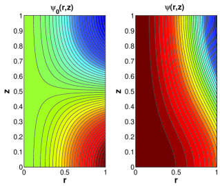
Figure 1: (Color online) Contour plot of the stream function associated to the “Beltrami solution”for the parameters $A=3$, $B=2$, $C=2$, $\mu=1/2$, $\kappa=\pi$, and $\phi=0$. The left hand side corresponds to the homogeneous solution (41) and the right hand side to the sum of the homogeneous solution and the particular solution (39).

II.7.3 $f$ and $g$ linear

The case where both $f$ and $g$ are linear $g=C+D\psi$ and $f=A+B\psi$ is similar to the previous one. The equations are now

$$\sigma = A+B\psi,$$

$$-\Delta_{*}\psi = \xi=\left[\frac{B^{2}}{2y}+D\right]\psi+\frac{AB}{2y}+C\;.$$ (42)

Note that these equations are obtained by minimizing the second moment of angular momentum $I_{2}=\int\sigma^{2}dydz$ at fixed $E$, $H$, $\Gamma$ and $I$. They represent, therefore, the counterpart of the minimum enstrophy principle in 2D hydrodynamics, leading to a linear relationship between vorticity and stream function. Equation (42-b) is an inhomogeneous linear equation for $\psi$. The general solution is the sum of a special solution of the inhomogeneous equation superposed to the general solution of the homogeneous equation. Solutions of the homogeneous equation can be found by assuming separation of variable as previously $\psi=F(z)G(y)$. The solution for $F$ is $F(z)=\cos(\kappa z+\phi)$, where $\kappa$ and $\phi$ are two integration constants. Then, the equation for $G$ involves a supplementary term compared to the one in the previous section:

$$\frac{d^{2}G}{dy^{2}}+\left(\frac{B^{2}-\kappa^{2}}{2y}+D\right)G=0.$$ (43)

The two solutions of this equations can be expressed in terms of Whittaker function (see Gradshteyn and Ryzhik (1965), p. 1059) $W_{\lambda,\pm 1/2}(2\sqrt{-D}y)$, $\lambda=(B^{2}-\kappa^{2})/8D$. These function behave at infinity like $y^{\lambda}\exp(-y/2)$. Turning back to original variable, one can therefore express the general solution of equation (42) as

$$\psi_{0}=\mu W_{\lambda,\pm 1/2}(\sqrt{-D}r^{2})\cos(\kappa z+\phi),$$ (44)

where $C$ is an integration constant. Note that the negativeness of the coefficient $D$ is imposed by an asymptotical analysis of equation (43): when $y\rightarrow\infty$, we see that a positive coefficient $D$ would introduce an oscillatory, unphysical, behavior for $G$. Figure 2 shows a typical realization of this solution.

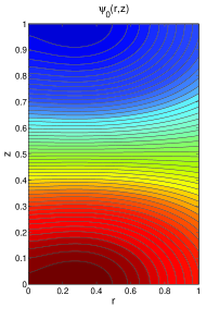
Figure 2: (Color online) Contour plot of the stream function associated to the “Whittaker solution”of equation (43) for the parameters $A=3$, $B=2$, $C=2$, $D=-3$, $\mu=1/2$, $\kappa=\pi$ and $\phi=0$.

III Statistical mechanics of axisymmetric flows

III.1 The mixing entropy

Starting with a given initial condition, equations (4) are expected to develop a complicated mixing process, with formation of finer and finer structure, leading to more and more degrees of freedom. A precise prediction of the state of the system would a priori require to keep track of all these degrees of freedom. Suppose however that we are only interested in the knowledge of the system at some coarse-grained scale. Since mixing is continuously occurring at smaller and smaller scales, we can expect the formation of a metaequilibrium state on the coarse-grained scale. Our goal is to derive its shape through thermodynamical arguments, based on entropy maximization in the spirit of Jaynes (1957). We focus here on basics. More discussion about this procedure can be found in Robert and Sommeria (1991). We introduce coarse-grained and fine-grained quantities. According to Eq. (4-c), $\psi=\Delta_{*}^{-1}\xi$ is expressed as an integral over $\xi$. It is therefore a smooth function whose fluctuations can be neglected $\psi=\overline{\psi}$. We shall determine the distribution of fluctuations of angular momentum $\sigma$ by an approach similar to that developed in 2D turbulence. We then introduce $\rho({\bf r},\eta)$, the density probability of finding the value $\sigma=\eta$ at position ${\bf r}$. Then, the coarse-grained angular momentum is $\overline{\sigma}=\int\rho\eta d\eta$ and the local normalization $\int\rho d\eta=1$. We introduce the mixing entropy

$$S[\rho]=-\int\rho\ln\rho\;dy\,dz\;d\eta\;.$$ (45)

This functional $S[\rho]$ is equal to the logarithm of the disorder where the disorder is the number of microstates corresponding to the macrostate $\rho({\bf r},\eta)$ which can be obtained by a combinatorial analysis (see Chavanis (2006) for details). The fact that the entropy depends only on the distribution of angular momentum guarantees that it will be conserved by the fine-grained dynamics (however, it increases on a coarse-grained scale as we will show subsequently). As a drawback, we will not be able to characterize the fluctuations of pseudo-vorticity $\xi$ by this method; we will simply get its coarse-grained value. This difficulty may reflect the fact that we are in a situation intermediate between 2D and 3D turbulence. In 2D turbulence, the distribution of vorticity is enough to construct equilibrium solutions whereas, in 3D turbulence, it is well-known that the average of fluctuating quantities (such as the Reynolds stress) are very important. In Appendix D, we consider another approach which puts the fluctuations of $\sigma$ and $\xi$ on an equal footing. This approach seems to indicate that the fluctuations of $\xi$ have a peculiar behavior that may give rise to a sort of “phase transition”. Here, for simplicity and clarity, we first concentrate on the simplified situation (similar to 2D turbulence) where the fluctuations of $\xi$ are mild; however, we keep in mind that there may be another regime (closer to 3D turbulence) characterizing axisymmetric flows.

The coarse-grained values of the constraints can be written as

$$\overline{E} = \frac{1}{2}\int\xi\psi\,dydz\;+\;\frac{1}{4}\int\frac{\overline{\sigma}^{2}}{y}\,dydz\;,$$ (46)

$$\overline{H} = \int\xi\,\overline{\sigma}\,dydz\;,\qquad\Gamma=\int\xi\,dydz\;,$$ (48)

$$\overline{I_{n}}=\int\rho\eta^{n}\;dydz\,d\eta\;.$$

For the coarse-grained energy, we made the non trivial hypothesis that the fluctuations of the energy could be neglected and used the coarse-grained field $\overline{\sigma}$ to calculate the mean energy. This is justified by the remark made in section II.5 that in the presence of a small viscosity (or a coarse-graining), the energy is approximately conserved.

As indicated previously, $E$, $\Gamma$, $H$ and $I$ are robust constraints. Thus they can be determined at any time since their exact value is close to their coarse-grained value. They have thus been expressed directly in terms of the coarse-grained field. By contrast the higher moments $I_{n>1}$ are fragile constraints because they are altered by coarse-graining. They can be determined only from the initial conditions which are supposed un-mixed (or from the fine-grained field) since they are affected by coarse-graining in the sense that $I_{n>1}[\overline{\sigma}]=\int\overline{\sigma}^{n}dydz\neq\overline{I_{n>1}[{\sigma}]}=\int\overline{\sigma^{n}}dydz=\int\rho\eta^{n}dydzd\eta$. Part of the Casimirs goes into the coarse-grained field and part goes into fine-grained fluctuations. In a sense, $I_{n>1}$ are “hidden constraints” because they cannot be determined from the coarse-grained field. Therefore, the statistical theory assumes that we know the initial conditions in detail and that these initial conditions represent the fine-grained field. This poses a conceptual problem because in real situations we are not sure whether the initial condition is already mixed or not. Furthermore, if the initial condition already results from a mixing process (like vortices formed in a succession of mergings in 2D decaying turbulence), it is more proper to ignore its fine structure and take its coarse-grained density as a new “fine-grained” initial condition to predict the next merging (see Chavanis and Sommeria (1996), p 284). In fact, due to viscosity, the fine structure of the field is progressively erased. These difficulties are intrinsic to the statistical theory of continuous fields.

III.2 The Gibbs state

The most probable distribution at metaequilibrium is obtained by maximizing the mixing entropy $S[\rho]$ at fixed $\overline{E}$, $\overline{H}$, $\overline{\Gamma}$, $\overline{I}$, $\overline{I_{n}}$ and normalization. We introduce Lagrange multipliers and write the variational principle in the form

$$\delta S-\beta\delta\overline{E}-\mu\delta\overline{H}-\gamma\delta\overline{\Gamma}-\alpha\delta\overline{I}-\sum_{n>1}\alpha_{n}\delta\biggl{(}\int\rho\eta^{n}\,dydzd\eta\biggr{)}$$ (49)

$$-\int\zeta(y,z)\delta\biggl{(}\int\rho d\eta\biggr{)}\,dydz=0\;.$$

The last term in this equation corresponds to the normalization of the probability density in each point of space and thus needs the introduction of one Lagrange multiplier $\zeta(y,z)$ for each point $(y,z)$. We shall treat the variations on $\rho$ and $\xi$ independently. The variations on $\xi$ imply

$$\beta\psi=-\mu\overline{\sigma}-\gamma.$$ (50)

The variations on $\rho$ yield the Gibbs state

$$\rho=\frac{1}{Z(y,z)}\chi(\eta)e^{-(\beta\frac{\overline{\sigma}}{2y}+\mu\xi+\alpha)\eta}\;,$$ (51)

where

$$\chi(\eta)=e^{-\sum_{n>1}\alpha_{n}\eta^{n}}.$$ (52)

To prepare the approach of Sec. III.5, we have distinguished between the Lagrange multipliers $\alpha_{n>1}$ which account for the conservation of the fragile constraints $I_{n>1}$ (they have been regrouped in the function $\chi(\eta)$) from the Lagrange multipliers $\beta$, $\mu$ and $\alpha$ which are related to the robust constraints. Therefore, the distribution (51) is the product of a universal Boltzmann factor and of a non-universal function $\chi(\eta)$ depending on the initial conditions. Note that instead of conserving the fine-grained moments $I_{n}=\int\overline{\sigma^{n}}dydz=\int\rho\eta^{n}d\eta dydz$ of angular momentum, we can equivalently conserve the total area $\gamma(\eta)=\int\rho dydz$ of each level. The “partition function” is determined by the local normalization condition yielding

$$Z=\int\chi(\eta)e^{-(\beta\frac{\overline{\sigma}}{2y}+\mu\xi+\alpha)\eta}d\eta.$$ (53)

We note that $Z$ is a function of

$$\Psi=\beta\frac{\overline{\sigma}}{2y}+\mu\xi+\alpha,$$ (54)

expressed by a sort of generalized Laplace transform (this is not exactly a Laplace transform since the variable $\eta$ can take positive and negative values):

$$Z(\Psi)=\int_{-\infty}^{+\infty}\chi(\eta)e^{-\eta\Psi}d\eta\equiv\hat{\chi}(\Psi).$$ (55)

The coarse-grained angular momentum is given by

$$\overline{\sigma}=\frac{1}{Z(\Psi)}\int\eta\chi(\eta)e^{-\eta\Psi}d\eta.$$ (56)

It is straightforward to establish that

$$\overline{\sigma}=-\frac{\partial\ln Z}{\partial\Psi}=F(\Psi)\qquad\text{and}\qquad\sigma_{2}=\frac{\partial^{2}\ln Z}{\partial\Psi^{2}}=-F^{\prime}(\Psi),$$ (57)

where

$$\sigma_{2}=\overline{(\sigma-\overline{\sigma})^{2}}=\overline{\sigma^{2}}-\overline{\sigma}^{2}\;,$$ (58)

is the centered variance of the local angular momentum distribution (we have noted $\overline{\sigma^{n}}=\int\rho\eta^{n}d\eta$). According to Eq. (57-b), $F$ is monotonically decreasing. Therefore, relation (57-a) can be inverted and we get

$$\beta\psi = -\mu\overline{\sigma}-\gamma\;,$$ (59)

$$\beta\frac{\overline{\sigma}}{2y} + \mu\xi+\alpha=F^{-1}(\overline{\sigma})\;.$$ (60)

Comparing with Eq. (11), we check explicitly that the coarse-grained flow is a stationary solution of the axisymmetric Euler equations. Therefore, for given initial conditions, the statistical theory selects a particular stationary solution among all possible ones. We remark that the differential equation for $\psi$, arising from Eq. (60) and (4)-c involves the inverse $F^{-1}$ of the function determined by Eq. (57-a) while in pure 2D turbulence it involves the direct function $F$, i.e. $-\Delta\psi=F(\beta\psi+\alpha)$. This “inversion” is another striking particularity of our system.

Comparing Eq. (60) with Eq. (24), we note that the equilibrium coarse-grained angular velocity maximizes a certain H-function where $C$ is related to $F$ by $F^{-1}(\overline{\sigma})=-C^{\prime}(\overline{\sigma})$, i.e.

$$C(\overline{\sigma})=-\int^{\overline{\sigma}}F^{-1}(x)dx\;.$$ (61)

The H-function $S[\overline{\sigma}]=-\int C(\overline{\sigma})d{\bf r}$ selected by the statistical theory can be viewed as a “generalized entropy” in the reduced $\overline{\sigma}$-space Chavanis (2003, 2005, 2005, 2006). It depends on the initial conditions through the function $\chi(\eta)$ which must be related to the fine-grained moments of angular momentum (Casimirs). Therefore, in this approach where the constraints associated with the Casimirs are treated microcanonically, the generalized entropy in $\overline{\sigma}$-space can only be obtained a posteriori, after having solved the full equilibrium equations and related the Lagrange multipliers to the constraints.

Using $\sigma_{2}=-\,d\,\overline{\sigma}/d\Psi$ according to (57)-b and $\Psi=-C^{\prime}(\overline{\sigma})$ according to (24)-b, we get the identity

$$\sigma_{2}=\frac{1}{C^{\prime\prime}(\overline{\sigma})}.$$ (62)

Therefore, at equilibrium, there is a functional relation between the variance $\sigma_{2}$ of the distribution and the coarse-grained angular momentum $\overline{\sigma}$ through the second derivative of the function $C$. This is similar to the “fluctuation-dissipation” theorem Chavanis and Sommeria (2002). Finally, we note that the most probable value $\langle\sigma\rangle(y,z)$ of the distribution $\rho(y,z,\eta)$ is such that ${\cal F}(\eta)=-\Psi\eta+\ln\chi(\eta)$ is maximum yielding $(\ln\chi)^{\prime\prime}<0$ and

$$\langle\sigma\rangle=[(\ln\chi)^{\prime}]^{-1}(\Psi)=G(\Psi),$$ (63)

where $G$ is monotonically decreasing. In general, the most probable value $\langle\sigma\rangle$ of the distribution (51) does not coincide with the mean value $\bar{\sigma}$. The condition $\langle\sigma\rangle=\bar{\sigma}$ is equivalent to

$$-(\ln\hat{\chi})^{\prime}=[(\ln\chi)^{\prime}]^{-1}.$$ (64)

This equality holds if $\chi$ is Gaussian. Furthermore, we show in Appendix C that $\langle\sigma\rangle$ is a stationary solution of the axisymmetric Euler equations only when $\langle\sigma\rangle=\overline{\sigma}$.

III.3 Particular cases

Some particular cases of $F(\Psi)$ relationships have been collected in Chavanis (2003, 2005, 2006). We shall specify different forms of function $\chi(\eta)$ and determine the corresponding $F(\Psi)$ and $S[\overline{\sigma}]$ from the preceding relations. We refer to Chavanis (2003) for more details. In the two-levels case where $\eta=\lambda_{0},\lambda_{1}$, we get

$$\overline{\sigma}=F(\Psi)=\lambda_{0}+\frac{\lambda_{1}-\lambda_{0}}{1+e^{(\lambda_{1}-\lambda_{0})\Psi}}.$$ (65)

In the present case, we need to invert this relation to express $\xi$ as a function of $\overline{\sigma}$, hence $\psi$. As discussed above, this situation is reversed with respect to pure 2D plane flows. We thus obtain

$$-\Delta_{*}\psi=\xi=\frac{1}{\mu(\lambda_{1}-\lambda_{0})}\ln\biggl{(}\frac{\mu\lambda_{1}+\beta\psi+\gamma}{-\beta\psi-\gamma-\lambda_{0}\mu}\biggr{)}+\frac{1}{2}\frac{\beta^{2}}{\mu^{2}}\frac{\psi}{y}+\frac{\beta\gamma}{2\mu^{2}y}-\frac{\gamma}{\mu}.$$ (66)

In that case, the generalized entropy in $\overline{\sigma}$-space has the form

$$S[\overline{\sigma}]=-\int[p\ln p+(1-p)\ln(1-p)]d{\bf r}\;,$$ (67)

with $\overline{\sigma}=p\lambda_{1}+(1-p)\lambda_{0}$. This is similar to the Fermi-Dirac entropy. In this two-levels case, the generalized entropy $S[\overline{\sigma}]$ defined by Eqs. (22)-(61) coincides with the mixing entropy $S[\rho]$ defined by Eq. (45). This is the only situation where we have this equivalence. Taking $\lambda_{0}=0$ and considering the dilute limit $\overline{\sigma}\ll\lambda_{1}$, we get

$$\overline{\sigma}=\lambda_{1}e^{-\lambda_{1}\Psi},$$ (68)

leading to

$$-\Delta_{*}\psi=\xi=-\frac{1}{\lambda_{1}\mu}\ln\biggl{(}\frac{-\beta\psi-\gamma}{\mu\lambda_{1}}\biggr{)}+\frac{1}{2}\frac{\beta^{2}}{\mu^{2}}\frac{\psi}{y}+\frac{\beta\gamma}{2\mu^{2}y}-\frac{\alpha}{\mu}.$$ (69)

In that case, the generalized entropy in $\overline{\sigma}$-space is similar to the Boltzmann entropy

$$S[\overline{\sigma}]=-\int\frac{\overline{\sigma}}{\lambda_{1}}\ln\frac{\overline{\sigma}}{\lambda_{1}}d{\bf r}.$$ (70)

If $\chi(\eta)$ is a Gaussian, then

$$\overline{\sigma}=-\sigma_{2}\Psi,$$ (71)

where the centered variance $\sigma_{2}$ is a constant. Inverting this relation, we get

$$-\Delta_{*}\psi=\xi=\frac{\beta}{\mu^{2}\sigma_{2}}\psi+\frac{\gamma}{\mu^{2}\sigma_{2}}+\frac{1}{2}\frac{\beta^{2}}{\mu^{2}}\frac{\psi}{y}+\frac{\beta\gamma}{2\mu^{2}y}-\frac{\alpha}{\mu}.$$ (72)

This is the type of mean-field equations that we have considered in Sec. II.7. In that case, the generalized entropy in $\overline{\sigma}$-space is

$$S[\overline{\sigma}]=-\frac{1}{2\sigma_{2}}\int\overline{\sigma}^{2}d{\bf r},$$ (73)

which is similar to minus the enstrophy in pure 2D hydrodynamics.

If $\chi(\eta)$ is a decentered Gamma distribution Ellis et al. (2002)-Chavanis (2006), then

$$\overline{\sigma}=-\frac{\sigma_{2}\Psi}{1+\lambda\sigma_{2}\Psi}\;,$$ (74)

where the centered variance $\sigma_{2}$ is a constant and $2\lambda\sigma_{2}^{1/2}$ is equal to the skewness of $\chi(\eta)$. Inverting this relation, we get

$$-\Delta_{*}\psi=\xi=\frac{\beta\psi+\gamma}{\sigma_{2}\mu(1-\lambda\beta\psi-\lambda\gamma)}+\frac{1}{2}\frac{\beta^{2}}{\mu^{2}}\frac{\psi}{y}+\frac{\beta\gamma}{2\mu^{2}y}-\frac{\alpha}{\mu}\;.$$ (75)

In that case, the generalized entropy in $\overline{\sigma}$-space is

$$S[\overline{\sigma}]=-\frac{1}{\lambda\sigma_{2}}\int\biggl{[}\overline{\sigma}-\frac{1}{\lambda}\ln(1+\lambda\overline{\sigma})\biggr{]}d{\bf r}.$$ (76)

III.4 Relaxation towards the statistical equilibrium state

We would like now to construct a system of relaxation equations which conserve all the invariants of the inviscid dynamics (robust and fragile) and relax towards the statistical equilibrium state. These equations can be used as a numerical algorithm to construct the statistical equilibrium state. They also provide a subgrid scale parameterization of axisymmetric turbulence. In that context, they can describe the dynamical evolution of the flow on the coarse-grained scale. Note that in the coarse-grained formulation, the inviscid approximation is easier to justify, since viscosity only acts at very small scales. Following the approach of Robert & Sommeria Robert and Sommeria (1992), these relaxation equations can be obtained by using a Maximum Entropy Production Principle (MEPP).

The equations of evolution for the coarse-grained fields are given by

$$\frac{\partial\overline{\sigma}}{\partial t}+\overline{\bf u}\cdot\nabla\overline{\sigma} = -\nabla\cdot{\bf J}_{\sigma}\;,$$ (77)

$$\frac{\partial\xi}{\partial t}+\overline{\bf u}\cdot\nabla{\xi} = \frac{\partial}{\partial x}\biggl{(}\frac{{\overline{\sigma}}^{2}}{4y^{2}}\biggr{)}-\nabla\cdot{\bf J}_{\xi}\;,$$

where ${\bf J}_{\sigma}$ and ${\bf J}_{\xi}$ are currents which contain all the information coming from interaction with sub-grid scales. Note that we have kept the advective terms because these equations are expected to describe the relaxation of the flow (on the coarse-grained scale) towards statistical equilibrium; they are not only numerical algorithms. If we want to keep track of the conservation of all the Casimirs (or equivalently of the total area of each level of angular momentum), we need to introduce equations of conservation for the density probability $\rho({\bf r},\eta,t)$ of angular momentum. We write them as

$$\frac{\partial\rho}{\partial t}+\overline{\bf u}\cdot\nabla\rho=-\nabla\cdot{\bf J}\;,$$ (78)

where ${\bf J}({\bf r},\eta,t)$ is the current of the level $\eta$ of angular momentum. Multiplying Eq. (78) by $\eta$ and integrating over all the levels, we recover Eq. (77-a) with ${\bf J}_{\sigma}=\int{\bf J}\,\eta\;d\eta$. Furthermore, the conservation of the local normalization $\int\rho\,d\eta=1$ imposes

$$\int{\bf J}\;d\eta=0.$$ (79)

The time variations of $S[\rho]$ are given by

$$\dot{S}=-\int{\bf J}\cdot\nabla\ln\rho\;d{\bf r}d\eta,$$ (80)

while the time variations of $E$ and $H$ have been given previously in Eqs. (27)-(28). Following the MEPP, we maximize $\dot{S}$ with $\dot{E}=\dot{H}=0$, the normalization constraint (79) and the additional constraints

$$\int\frac{J^{2}}{2\rho}d\eta\leq C({\bf r},t),\qquad\frac{J_{\xi}^{2}}{2}\leq C_{\xi}({\bf r},t).$$ (81)

Writing the variational principle in the form

$$\delta\dot{S}-\beta\delta\dot{E}-\mu\delta\dot{H}-\int\zeta\delta\biggl{(}\int{\bf J}d\eta\biggr{)}d{\bf r}-\int{\chi}\delta\biggl{(}\frac{J^{2}}{2\rho}\biggr{)}d{\bf r}d\eta-\int{\chi^{\prime}}\delta\biggl{(}\frac{J_{\xi}^{2}}{2\xi}\biggr{)}d{\bf r}=0,$$ (82)

we obtain the optimal currents

$${\bf J} = -D\biggl{[}\nabla\rho+\frac{1}{2}\beta\rho(\eta-\overline{\sigma})\nabla\biggl{(}\frac{\overline{\sigma}}{y}\biggr{)}+\mu\rho(\eta-\overline{\sigma})\nabla\xi\biggr{]},$$ (83)

$${\bf J}_{\xi} = -D^{\prime}(\beta\nabla\psi+\mu\nabla\sigma),$$ (84)

where we have used Eq. (79) to obtain the final expression of the current (83). The current of angular momentum is therefore given by

$${\bf J}_{\sigma}=-D\biggl{[}\nabla\overline{\sigma}+\frac{1}{2}\beta\sigma_{2}\nabla\biggl{(}\frac{\overline{\sigma}}{y}\biggr{)}+\mu\sigma_{2}\nabla\xi\biggr{]},$$ (85)

where $\sigma_{2}$ is defined in Eq. (58). We note that $\beta(t)$ and $\mu(t)$ are time dependent Lagrange multipliers that evolve in order to conserve energy and helicity. Their explicit expression is obtained by inserting Eqs. (84) and (85) in the constraints (27)-(28).

We now show that the relaxation equations (77-b) and (78) with the currents (84) and (83) increase the mixing entropy (45) until the Gibbs state is reached ($H$-theorem). We can write the rate of entropy production (80) in the form

$$\dot{S}=-\int\frac{{\bf J}}{\rho}\cdot\biggl{[}\nabla\rho+\frac{1}{2}\beta\rho(\eta-\overline{\sigma})\nabla\biggl{(}\frac{\overline{\sigma}}{y}\biggr{)}+\mu\rho(\eta-\overline{\sigma})\nabla\xi\biggr{]}\,d{\bf r}d\eta$$ (86)

$$+\frac{1}{2}\beta\int(\eta-\overline{\sigma}){\bf J}\cdot\nabla\biggl{(}\frac{\overline{\sigma}}{y}\biggr{)}\,d{\bf r}d\eta+\mu\int(\eta-\overline{\sigma}){\bf J}\cdot\nabla\xi\,d{\bf r}d\eta.$$

Using Eqs. (84) and (83) this can be rewritten

$$\dot{S}=\int\frac{{\bf J}^{2}}{D\rho}\,d{\bf r}+\frac{1}{2}\beta\int{\bf J}_{\sigma}\cdot\nabla\biggl{(}\frac{\overline{\sigma}}{y}\biggr{)}\,d{\bf r}+\mu\int{\bf J}_{\sigma}\cdot\nabla\xi\,d{\bf r}.$$ (87)

Using Eqs. (27)-(28), we get

$$\dot{S}=\int\frac{{\bf J}^{2}}{D\rho}d{\bf r}-\int{\bf J}_{\xi}\cdot(\beta\nabla\psi+\mu\nabla\overline{\sigma})d{\bf r},$$ (88)

hence

$$\dot{S}=\int\frac{{\bf J}^{2}}{D\rho}d{\bf r}+\int\frac{{\bf J}_{\xi}^{2}}{D^{\prime}}d{\bf r}.$$ (89)

We conclude that $\dot{S}\geq 0$ provided that $D,D^{\prime}>0$. At equilibrium $\dot{S}=0$ yielding ${\bf J}={\bf J}_{\xi}=0$. Equations (84) and (83) imply

$$\nabla\ln\rho+\frac{1}{2}\beta(\eta-\overline{\sigma})\nabla\biggl{(}\frac{\overline{\sigma}}{y}\biggr{)}+\mu(\eta-\overline{\sigma})\nabla\xi=0,$$ (90)

$$\beta\nabla\psi+\mu\nabla\overline{\sigma}=0.$$ (91)

The second equation is equivalent to

$$\overline{\sigma}=-\frac{\beta}{\mu}\psi-\frac{\nu}{\mu}.$$ (92)

On the other hand, for any reference level $\eta_{0}$, Eq. (90) yields

$$\nabla\ln\rho_{0}+\frac{1}{2}\beta(\eta_{0}-\overline{\sigma})\nabla\biggl{(}\frac{\overline{\sigma}}{y}\biggr{)}+\mu(\eta_{0}-\overline{\sigma})\nabla\xi=0.$$ (93)

Subtracting Eqs. (90)-(93) and integrating, we obtain

$$\ln\biggl{(}\frac{\rho}{\rho_{0}}\biggr{)}+\frac{1}{2}\beta(\eta-\eta_{0})\frac{\sigma}{y}+\mu(\eta-\eta_{0})\xi=A(\eta),$$ (94)

which can be written

$$\rho=\frac{1}{Z({\bf r})}\chi(\eta)e^{-(\beta\frac{\overline{\sigma}}{2y}+\alpha)\eta}e^{-\mu\xi\eta}.$$ (95)

Thus, the stationary solution of the relaxation equations is the Gibbs state (51).

The relaxation equations are relatively complicated to solve, because we need to solve $N$ coupled PDE, one for each level. Alternatively, we can write down a hierarchy of equations for the moments of angular momentum $\overline{\sigma^{n}}$. The first moment equations of the hierarchy can be written

$$\frac{\partial\overline{\sigma}}{\partial t}+{\bf u}\cdot\nabla\overline{\sigma} = \nabla\cdot\biggl{\{}D\biggl{[}\nabla\overline{\sigma}+\frac{1}{2}\beta\sigma_{2}\nabla\biggl{(}\frac{\overline{\sigma}}{y}\biggr{)}+\mu\sigma_{2}\nabla\xi\biggr{]}\biggr{\}},$$ (96)

$$\frac{\partial\xi}{\partial t}+{\bf u}\cdot\nabla{\xi} = \frac{\partial}{\partial z}\biggl{(}\frac{{\overline{\sigma}}^{2}}{4y^{2}}\biggr{)}+\nabla\biggl{[}D^{\prime}(\beta\nabla\psi+\mu\nabla\overline{\sigma})\biggr{]}.$$ (97)

We are now led to a complicated closure problem because each equation of the hierarchy involves the next order moments. For example, the equation for $\overline{\sigma}$ involves $\sigma_{2}$ etc. In the two levels approximation, one has $\sigma_{2}=(\overline{\sigma}-\lambda_{0})(\lambda_{1}-\overline{\sigma})$. On the other hand, a Gaussian distribution of fluctuations at equilibrium can be obtained by imposing that $\sigma_{2}$ is constant. In these two particular cases, the equations (96) are closed. More generally, we must write down the higher moments of the hierarchy and close them with a local maximum entropy principle as proposed by Robert & Rosier Robert and Rosier (1997). If we implement this procedure up to second moment, it leads to a Gaussian distribution. Its implementation to higher moments is difficult. Furthermore, its physical justification is unclear. In practice, we must come back to the $N$ coupled PDE for the levels.

III.5 Prior distribution and generalized entropy

In the statistical approach presented previously, we have assumed that the system is rigorously described by the axisymmetric Euler equations so that the conservation of all the Casimirs $I_{n}$ must be taken into account. This corresponds to a freely evolving situation. Alternatively, in the case of flows that are forced at small-scales, Ellis et al. Ellis et al. (2002) have proposed to replace the conservation of all the Casimirs by the specification of a prior distribution $\chi(\eta)$ encoding the small-scale forcing. This approach has been further developed in Chavanis Chavanis (2005). In this approach, the constraints associated with the (fragile) moments $I_{n>1}$ are treated canonically instead of microcanonically. By contrast, the robust constraints (energy, circulation, helicity, angular momentum) are still treated microcanonically. If we view the levels $\eta$ of angular momentum as different species of particles, this approach amounts to fixing the chemical potentials instead of the total number of particles in each species. The idea is that the ambient medium behaves as a reservoir of angular momentum: the small-scale forcing and dissipation affect the conservation of the moments of angular momentum $I_{n>1}$ while fixing instead the canonical variables $\alpha_{n}$.

Therefore, in the present situation, the relevant entropy $S_{\chi}$ is obtained from the mixing entropy (45) by making a Legendre transform on the fragile moments $I_{n>1}$ Chavanis (2005). If we assume that the $\alpha_{n}$ in the variational principle (49) are fixed by the “reservoir” (ambient medium), we can define a relative entropy by

$$S_{\chi}=S-\sum_{n>1}\alpha_{n}\overline{I_{n}}=S-\sum_{n>1}\alpha_{n}\int\rho\eta^{n}\,dydzd\eta.$$ (98)

This is similar to the passage from the entropy $S$ (microcanonical description) to the grand potential $\Omega=S-\mu N$ (grand microcanonical description) in usual thermodynamics when the chemical potential is fixed instead of the particle number. Using Eq. (45), we get

$$S_{\chi}=-\int\rho\biggl{[}\ln\rho+\sum_{n>1}\alpha_{n}\eta^{n}\biggr{]}\,dydzd\eta.$$ (99)

Introducing the function (52), we obtain

$$S_{\chi}=-\int\rho\ln\biggl{[}\frac{\rho}{\chi(\eta)}\biggr{]}\,dydzd\eta.$$ (100)

The function $\chi(\eta)$ is interpreted as a prior distribution of angular momentum. It is a global distribution of angular momentum fixed by the small-scale forcing. It must be regarded as given. In this approach, the statistical equilibrium state is obtained by maximizing the relative entropy (100) while conserving only the robust constraints. Thus, we write the variational problem as

$$\delta S_{\chi}-\beta\delta E-\mu\delta H-\gamma\delta\Gamma-\alpha\delta I-\int\zeta(y,z)\delta\biggl{(}\int\rho d\eta\biggr{)}dydz=0.$$ (101)

We can now repeat the calculations of Sec. III.2 with almost no modification. The only difference is that we regard the $\alpha_{n}$’s as given. Therefore, the Gibbs state is determined by Eq. (51) where $\chi(\eta)$ is fixed a priori by the small-scale forcing. Recall that in the previous approach (freely evolving flows), it had to be determined a posteriori from the initial conditions (assumed known) by a complicated procedure. Here, the specification of $\chi(\eta)$ automatically determines the function $F$ by Eq. (57) and then $C$ by Eq. (61). Thus, the generalized entropy in $\overline{\sigma}$-space $S[\overline{\sigma}]=-\int C(\overline{\sigma})\,d{\bf r}$ is now determined by the small-scale forcing through the prior $\chi(\eta)$ while in the preceding approach it was determined by the initial conditions through the Casimirs $I_{n>1}$. Explicitly, the generalized entropy is expressed as a function of $\chi$ by the formula Chavanis (2006):

$$C(\overline{\sigma})=-\int^{\overline{\sigma}}[(\ln\hat{\chi})^{\prime}]^{-1}(-x)dx.$$ (102)

The equilibrium coarse-grained angular momentum $\overline{\sigma}$ maximizes the generalized entropy (22)-(102) at fixed robust constraints $E$, $\Gamma$, $H$ and $I$. In the present context, the relaxation equations introduced in Sec. II.6 can describe the relaxation of the coarse-grained flow towards statistical equilibrium once the small-scale forcing has established a permanent regime characterized by a prior distribution $\chi(\eta)$ determining a generalized entropy $S[\overline{\sigma}]$. Since we are now interested by the route to equilibrium we need to restore the advective terms, so we write:

$$\frac{\partial\overline{\sigma}}{\partial t}+{\bf u}\cdot\nabla\overline{\sigma} = \nabla\cdot\biggl{\{}D\biggl{[}\nabla\overline{\sigma}+\frac{\beta}{C^{\prime\prime}(\overline{\sigma})}\nabla\biggl{(}\frac{\overline{\sigma}}{2y}\biggr{)}+\frac{\mu}{C^{\prime\prime}({\overline{\sigma}})}\nabla\xi\biggr{]}\biggr{\}},$$ (103)

$$\frac{\partial\xi}{\partial t}+{\bf u}\cdot\nabla{\xi} = \frac{\partial}{\partial z}\biggl{(}\frac{{\overline{\sigma}}^{2}}{4y^{2}}\biggr{)}+\nabla\cdot\biggl{[}D^{\prime}(\beta\nabla\psi+\mu\nabla\overline{\sigma})\biggr{]}.$$

The physical interpretation of these equations is quite different from (33). In Sec. II.6, the relaxation equations (33) provide a numerical algorithm to determine any nonlinearly dynamically stable stationary solution of the axisymmetric equations, specified by the convex function $C$. In this context, only the stationary solution for $t\rightarrow+\infty$ matters and the evolution towards that state has no physical meaning (it is just the engine of the algorithm). In the present section, the relaxation equations (103) provide a description of the evolution of the coarse-grained field, for all time $t$, in a medium where a small-scale forcing imposes a prior distribution $\chi(\eta)$ (or a generalized entropy $C(\overline{\sigma})$ in the reduced $\overline{\sigma}$-space). These equations conserve only the robust constraints and satisfy a generalized maximum entropy production principle for the functional $S[\overline{\sigma}]$. Finally, the relaxation equations of Sec. III.4 provide a description of the evolution of the coarse-grained field, for all time $t$, of a freely evolving system. These equations conserve all the constraints (including the Casimirs) and satisfy a maximum entropy production principle for the functional $S[\rho]$. Note that the relaxation equations (103) can also be obtained from the moments equations (96)-(97) of the ordinary statistical theory by using the relation (62) to express $\sigma_{2}$ as a function of $\overline{\sigma}$. In a sense, this relation can be seen as a closure relation imposed by a small-scale forcing. Thus, the relaxation equations (103) are not simply numerical algorithms; they can also provide a parameterization of axisymmetric flows with a small-scale forcing. Their interest as numerical algorithms (in the sense of Sec. II.6) remains however important in case of incomplete relaxation to construct stable stationary solutions of the Euler equation which are not consistent with the statistical theory (in cases where the evolution is non-ergodic) in order to reproduce the observations, as discussed in Chavanis (2003, 2005, 2005, 2006).

IV Summary

In this paper, we have developed new variational principles to study the structure and the stability of equilibrium axisymmetric flows. We have completely characterized the steady states of the inviscid dynamics and found that there is an infinite number of solutions. We have shown that each of these steady states extremizes a certain functional and that maxima or minima of this functional correspond to nonlinearly dynamically stable states. We have given analytical solutions in some simple cases to illustrate our formalism. One of these steady states (non-universal) will be reached on the coarse-grained scale as a result of violent relaxation (chaotic mixing). Our general approach must be contrasted from that of other authors who obtained particular solutions of the Navier-Stokes equation by means of phenomenological principles (minimum of enstrophy for example in 2D turbulence, Beltramization for MHD and axisymmetric flows,…). Such solutions are recovered as particular cases of our formalism but many other solutions can emerge in practice depending on the initial conditions, on the route to equilibrium (ergodicity) and on the type of forcing. This is why we try to remain very general. Our point is that there is no clear universality in 2D or axisymmetric turbulence Chavanis (2003, 2005, 2005, 2006). In a second part, we have developed a thermodynamical approach to determine the statistical equilibrium states at some fixed coarse-grained scale. We found that the resulting distribution can be divided in two parts: one universal part, coming from the robust constraints, and one non-universal, which depends on the initial conditions (Casimirs) for freely evolving systems or on a prior distribution encoding non-ideal effects such as forcing and dissipation. Finally, we have derived relaxation equations which can be used either as numerical algorithm to compute stable stationary solutions of the axisymmetric Euler equations, or to describe the dynamics of the system (freely evolving or forced) at the coarse-grained level.

The main question regarding the application of our results to realistic systems (such as the ones mentioned in the Introduction) is the relevance of the use of the ideal (Euler) equation instead of the true dissipative system. In fact, the presence of a small viscosity does not preclude the applicability of our results. First of all, since viscosity acts at small scales, its main effect is to erase the fluctuations around the coarse-grained field. Thus, it gives a physical support for selecting the coarse-grained field which is at large scales and which is relatively robust against viscosity. On the other hand, we have shown that viscosity and coarse-graining act in a similar manner so that they are not in opposition. In a very turbulent flow, the diffusion acts only at small scales by dissipating energy. By disregarding the details of the fine-grained dynamics, we have a similar process where energy is lost in the small-scales but accumulates in the large-scales. On the other hand, we have shown that a (generalized) selective decay principle can be motivated either by viscous effects or by coarse-graining. Indeed, a small viscosity or a coarse-graining tend to increase the value of the $H$-functions (fragile constraints) with only weak modification on the energy, angular momentum, circulation and helicity (robust constraints). Therefore, viscous effects do not break the nonlinear dynamical stability results. On the contrary, they can precisely explain (together with coarse-graining) how the system can reach a maximum of an $H$-function at fixed robust constraints. Without dissipation (viscosity or coarse-graining) this is not possible since the Casimir functionals $S[\sigma]$ are rigorously conserved by the Euler equation. We believe, however, that the main increase of the fragile constraints (like enstrophy) is due to coarse-graining Chavanis and Sommeria (1996) rather than molecular viscosity (in classical works on 2D turbulence, it is argued instead that enstrophy is dissipated essentially by viscosity). The main difference between viscous and inviscid flows is that inviscid flows tend to a strict stationary solution of the Euler equation (on the coarse-grained scale) while, in the presence of a small viscosity, this large-scale structure slowly diffuses and ultimately disapears. However, if $\nu\rightarrow 0$, this happens on a long time scale that is not of most physical interest. Note finally that forcing can act against viscosity and maintain a steady state as for an inviscid evolution.

The other effect of viscosity, now regarding the statistical mechanics approach, is to break the conservation of the Casimirs. This is a problem for the original approach (Sec. III.2) where it is assumed that all the Casimirs are conserved. However, in the point of view developed in Sec. III.5, we have replaced the specification of the Casimirs by a prior distribution of angular momentum. It corresponds to the non-universal part of the distribution of fluctuations given by the Gibbs state (51). We have argued that this prior is precisely determined by non-ideal effects such as viscosity and forcing (in addition to the initial conditions and the boundary conditions), i.e. by all the complicated features of turbulence. Therefore, in this point of view, the existence of a viscosity and a forcing can be taken into account phenomenologically in the theory. On the other hand, it should be noted that the effect of coarse-graining is similar to a turbulent viscosity. This is best seen in the relaxation equations (103) which involve a diffusion term with a “turbulent viscosity” $D$. However, our approach shows that the adjunction of a turbulent viscosity to the Euler equations in order to model turbulence is not sufficient as it breaks the conservation of energy. Therefore, additional drift terms arise in the relaxation equations to act against diffusion and lead to a steady state Chavanis (2005). There are other pieces of evidence for the claim that the introduction of a coarse-graining procedure is similar to a diffusive process. For example, recent numerical simulations have shown that the Euler equation with a high wave-number spectral truncation shows similar features as the Navier-Stokes (dissipative) equation Cichowlas et al. (2005). This issue concerning the influence of viscosity will be addressed more thoroughly in a second paper, where we confront our prediction to experimental data, and use them to derive and characterize the non-universal features of the equilibrium distributions.

Finally, we will address the changes to be made to account for a global rotation of the system. Taking the rotation vector to be aligned in the $z$-direction, the Coriolis force will only add a term $2\Omega u$ on the left-hand-side of the first equation (2). Then, the conserved quantity will be $\sigma^{\prime}=rv+\Omega r^{2}$ instead of $\sigma=rv$. This is similar to the use of a potential vorticity when doing the statistical mechanics of two-dimensional rotating fluid instead of the usual vorticity Chavanis and Sommeria (2002). Similarly, the right-hand side of the second equation will now be: $\partial_{z}[(v^{2}+2\Omega vr)/r]=\partial_{z}[(v^{2}+2\Omega vr+\Omega^{2}r^{2})/r]=\partial_{z}[\sigma^{\prime 2}/r^{3}]$. Consequently, all the results in this paper will be valid provided that $\sigma^{\prime}$ is used instead of $\sigma$.

Appendix A Derivation of conservation laws

In this Appendix, we prove the conservation laws used in the main text. A cornerstone of the proof is the general identity:

$$\int\chi\{\phi,\psi\}\,dydz=-\int\phi\{\chi,\psi\}\,dydz\;,$$ (104)

which holds if one of the two fields $\chi$ or $\phi$ vanishes on the boundary of the domain.

• Energy conservation: using the equations of motion and assuming that $\psi=0$ or $\xi=\sigma=0$ on the boundary of the domain, we have

  $$\dot{E} = \int\psi\frac{\partial\xi}{\partial t}\,dydz+\int\frac{\sigma}{2y}\frac{\partial\sigma}{\partial t}\,dydz,$$

  $$= \int\psi\left[-\{\psi,\xi\}-\{\frac{\sigma}{2y},\sigma\}\right]-\frac{\sigma}{2y}\{\psi,\sigma\}\,dydz$$

  $$= \int\left(-\xi\{\psi,\psi\}+\frac{\sigma}{2y}\{\psi,\sigma\}-\frac{\sigma}{2y}\{\psi,\sigma\}\right)\,dydz$$

  $$= 0,$$

  where we have used the identity (104) twice to obtain the third line.

• Casimirs conservation: using the equations of motion and $\psi=0$ or $\sigma=0$ on the boundary, we will show that all the moments of $\sigma$ are conserved:

  $$\dot{I}_{n} = n\int\sigma^{n-1}\frac{\partial\sigma}{\partial t}\,dydz\,,$$

  $$= -n\int\sigma^{n-1}\{\psi,\sigma\}\,dydz$$

  $$= n\int\psi\{\sigma^{n-1},\sigma\}\,dydz$$

  $$= 0,$$

  where we have used the identity (104) in the third line.

• Helicity conservation: using the equations of motion, we have

  $$\dot{H} = \int\biggl{\{}F(\sigma)\frac{\partial\xi}{\partial t}+\xi F^{\prime}(\sigma)\frac{\partial\sigma}{\partial t}\biggr{\}}\,dydz\,,$$

  $$= -\int F(\sigma)\biggl{[}\{\psi,\xi\}+\{\frac{\sigma}{2y},\sigma\}\biggr{]}-\int\xi F^{\prime}(\sigma)\{\psi,\sigma\}\,dydz\,.$$

  Then,

  $$\int F(\sigma)\{\frac{\sigma}{2y},\sigma\}\,dydz=-\int\frac{\sigma}{2y}\{F(\sigma),\sigma\}\,dydz=0\;,$$ (108)

  if $\sigma$ or $F(\sigma)$ vanishes on the boundary of the domain. Therefore,

  $$\dot{H} = -\int F(\sigma)\{\psi,\xi\}dydz-\int\xi F^{\prime}(\sigma)\{\psi,\sigma\}\,dydz$$

  $$= -\int F(\sigma)\{\psi,\xi\}\,dydz+\int\xi\{F(\sigma),\psi\}\,dydz$$

  $$= -\int\xi\{F(\sigma),\psi\}\,dydz+\int\xi\{F(\sigma),\psi\}\,dydz$$

  $$= 0,$$

  where we have used identity (8) in the second line and identity (104) in the third line and assumed that $F(\sigma)=0$ or $\xi=0$ on the boundary of the domain.

Appendix B Stability of solutions

In section II.4, we found that the functions $\sigma_{0}(y,z)$ and $\xi_{0}(y,z)$ which extremize the functional (22) are solutions of the following set of equations :

$$\beta\psi_{0}=-\mu\sigma_{0}-{\nu}\qquad\mathrm{and}\qquad-C^{\prime}(\sigma_{0})={\beta}\frac{\sigma_{0}}{2y}+\mu\xi_{0}+\alpha.$$ (110)

However, only maxima of $S$ are nonlinearly dynamically stable. We need therefore to investigate the sign of the second order variations of $J=S-\beta E-\mu H-\nu\Gamma-\alpha I$. Writing $\sigma=\sigma_{0}+\delta\sigma$, $\xi=\xi_{0}+\delta\xi$ and $\psi=\psi_{0}+\delta\psi$, one obtains for all $\delta\sigma$ and $\delta\xi$:

$$\delta^{2}J[\sigma_{0},\xi_{0}]=-\int dydz\;\left[\left(C^{\prime\prime}(\sigma_{0})+\frac{\beta}{2y}\right)(\delta\sigma)^{2}+2\mu\delta\sigma\delta\xi+\beta\delta\psi\delta\xi\right]\;,$$ (111)

with $\delta\xi=-\Delta_{*}\delta\psi$. Using the operators $curl$ and ${\bf Curl}$ defined in Leprovost et al. (2005), one can easily show that the last term can be rewritten :

$$\beta\int\delta\psi\delta\xi\;dydz=\beta\int\left[{\bf Curl}\left(\frac{\delta\psi}{r}\right)\right]^{2}\;dydz\;.$$ (112)

Putting $\delta\sigma=0$ in equation (111), the condition $\delta^{2}J[\sigma_{0},\xi_{0}]<0$ thus implies that $\beta$ must be positive. This is at variance with pure 2D hydrodynamics, where stable structures can exist at negative temperature and are the most relevant. Also, assuming $\delta\xi=0$, one finds that a maximum of $J$ should satisfy the following condition:

$$\int\;\left(C^{\prime\prime}(\sigma_{0})+\frac{\beta}{2y}\right)(\delta\sigma)^{2}\;dydz>0\;,$$ (113)

which is trivially fulfilled because $C$ is a convex function. One cannot find a general condition on the value of $\mu$ in order for $\delta^{2}J[\sigma_{0},\xi_{0}]$ to be negative but a sufficient condition can be found by using the fact that in (111), the last term in the integral is everywhere positive. Consequently, a sufficient condition for $\delta^{2}J<0$ is:

$$\int dydz\;\left[\left(C^{\prime\prime}(\sigma_{0})+\frac{\beta}{2y}\right)(\delta\sigma)^{2}+2\mu\delta\sigma\delta\xi\right]>0$$ (114)

$$\Leftrightarrow\int dydz \left[\left(C^{\prime\prime}(\sigma_{0})+\frac{\beta}{2y}\right)\left(\delta\sigma+\frac{\mu}{C^{\prime\prime}(\sigma_{0})+\frac{\beta}{2y}}\delta\xi\right)^{2}-\frac{\mu^{2}}{\left(C^{\prime\prime}(\sigma_{0})+\frac{\beta}{2y}\right)^{2}}(\delta\xi)^{2}\right]>0\;,$$

for all $\delta\sigma$ and $\delta\xi$. This condition can obviously be provided if $\mu=0$. A sufficient condition for $\sigma_{0}$ and $\xi_{0}$, solution of (110), to be maximum of $S$ is thus $\mu=0$ and $\beta>0$. However, this is only a very particular case.

Appendix C Stationarity of $\langle\sigma\rangle$

The most probable value of the distribution (51) can be written

$$\langle\sigma\rangle=G(\Psi)=G[F^{-1}(\bar{\sigma})]=G\Bigl{[}F^{-1}\bigl{(}-\frac{\beta\psi+\gamma}{\mu}\bigr{)}\Bigr{]}\;,$$ (115)

showing that $\langle\sigma\rangle=f(\psi)$ is a function of $\psi$ alone. We now write the condition under which $\langle\sigma\rangle$ is a stationary solution of the axisymmetric Euler equations. Comparison between Eqs. (14) and (60) shows that the following relation must hold :

$$-\frac{\beta}{\mu}\bar{\sigma}=\frac{1}{2}\frac{d}{d\psi}f^{2}.$$ (116)

Using Eq. (59), this can be rewritten:

$$f(\psi)=\sqrt{\frac{\beta^{2}\psi^{2}}{\mu^{2}}+2\frac{\gamma\beta}{\mu^{2}}\psi+c}\;,$$ (117)

where $c$ is an integration constant. If we require that $\bar{\sigma}=\langle\sigma\rangle$ on the boundary of the domain ($\psi=0$), then, using Eq. (59), we get $f^{2}(0)=c={\gamma^{2}}/{\mu^{2}}$. Substituting in Eq. (117), we find that $G\circ F^{-1}$ is the identity so that $\langle\sigma\rangle=\bar{\sigma}$ (everywhere). This implies that $\langle\sigma\rangle$ is a stationary solution of the axisymmetric equations only when it coincides with $\bar{\sigma}$ .

Appendix D Fluctuations of $\xi$

D.1 Generalities

In this Appendix, we try to develop the statistical mechanics approach in the general case, without ignoring the fluctuations of $\xi$. Since $\xi$ is not conserved by the axisymmetric equations ($D\xi/Dt\neq 0$), this may invalidate the use of a statistical theory to predict its fluctuations, so that our approach is essentially phenomenological and explanatory. We introduce $\rho({\bf r},\eta,\nu)$, the density probability of finding the values $\sigma=\eta$ and $\xi=\nu$ in ${\bf r}$ at equilibrium. Then, the coarse-grained fields are $\overline{\sigma}=\int\rho\eta\,d\eta d\nu$, $\overline{\xi}=\int\rho\nu\,d\eta d\nu$ and the local normalization is $\int\rho\,d\eta d\nu=1$. We introduce the mixing entropy

$$S[\rho]=-\int\rho\ln\rho\ dydzd\eta d\nu.$$ (118)

As usual, the fluctuations of $\psi$ will be neglected because it is an integrated quantity of the primitive field $\xi$. The integral constraints can be re-expressed as

$$\overline{E} = \frac{1}{2}\int\rho\nu\psi\;dydzd\eta d\nu\,+\,\frac{1}{4}\int\rho\frac{\eta^{2}}{y}\;dydzd\eta d\nu\;,$$ (120)

$$\overline{H_{n}}=\int\rho\nu\eta^{n}\;dydzd\eta d\nu\;,$$

$$\overline{I_{n}} = \int\rho\eta^{n}\;dydzd\eta d\nu,\;,\qquad\overline{\Gamma}=\int\rho\nu\;dydzd\eta d\nu.\;$$ (121)

The most probable distribution at metaequilibrium is therefore obtained by maximizing the entropy at fixed $E$, $H_{n}$ and $I_{n}$. We introduce Lagrange multipliers and write the variational principle in the form

$$\delta S-\beta\delta\overline{E}-\sum_{n}\mu_{n}\delta\overline{H_{n}}-\sum_{n}\alpha_{n}\delta\overline{I_{n}}-\int\zeta(y,z)\delta\biggl{(}\int\rho\;d\eta d\nu\biggr{)}\;dydz=0.$$ (122)

The variations on $\rho$ yield the Gibbs state

$$\rho=\frac{1}{Z(y,z)}e^{-\beta[\nu\psi+\frac{\eta^{2}}{4y}]-\alpha G(\eta)-\mu F(\eta)\nu},$$ (123)

where $\mu F(\eta)=\sum_{n}\mu_{n}\eta^{n}$ and $\alpha G(\eta)=\sum_{n}\alpha_{n}\eta^{n}$ . The “partition function” is determined by the local normalization condition yielding

$$Z=\int e^{-\beta[\nu\psi+\frac{\eta^{2}}{4y}]-\alpha G(\eta)-\mu F(\eta)\nu}d\eta d\nu.$$ (124)

The coarse-grained fields $\bar{\sigma}$ and $\bar{\xi}$ are the averaged values of the distribution (123). This approach predicts that the distribution of fluctuations of pseudo-vorticity is exponential $\sim e^{\Lambda(y,z,\eta)\nu}$ so that, depending on the sign of $\Lambda$, it diverges either for $\nu\rightarrow+\infty$ or $\nu\rightarrow-\infty$. The problem of the smoothness of the vorticity is still an unresolved issue for the Navier-Stokes equation related to the existence and uniqueness of its solutions. In two dimensions, it can be shown that it is bounded Doering and Gibbon (1995) whereas in three dimensions, very little is known. In our case, which is intermediate between these two cases, we can infer that the vorticity will be bounded as we have seen that in the axisymmetric case, the vorticity has to vanish in the long time limit (see section II.5). The range of integration for the variable $\nu$ is thus restricted to finite values: $|\nu|<\lambda$.

We now look for extremum values of the distribution (123).To study this problem, we write:

$$\rho(y,z,\eta,\nu) = \frac{1}{Z}\exp[-\cal{F}(\eta,\nu)]\;,$$ (125)

$$\text{with}\qquad\cal{F} = \nu[\beta\psi+\mu F(\eta)]+\frac{\beta\eta^{2}}{4y}+\alpha G(\eta)\;.$$

We start to search for extrema of the distribution in the interior of the domain $]-\xi_{m},\xi_{m}[$ and call them $\langle\sigma\rangle,\langle\xi\rangle$. One can check that they obey the equations:

$$\frac{\partial{\cal F}}{\partial\eta}\Big{|}_{\langle\sigma\rangle,\langle\xi\rangle} = \frac{\beta\langle\sigma\rangle}{2y}+\alpha G\,^{\prime}(\langle\sigma\rangle)+\mu\langle\xi\rangle F\,^{\prime}(\langle\sigma\rangle)=0,$$ (126)

$$\frac{\partial{\cal F}}{\partial\nu}\Big{|}_{\langle\sigma\rangle,\langle\xi\rangle} = \beta\psi+\mu F(\langle\sigma\rangle)=0.$$

These extremum fields $\langle\sigma\rangle$ and $\langle\xi\rangle$ are stationary states of the Euler axisymmetric equation (with families indexed through the conservation laws) while the averaged states $\bar{\sigma}$ and $\bar{\xi}$ are not in general. The stability of these extremum states can be found in principle by considering the second variations of ${\cal F}$. Here, we prefer to use the following trick. We introduce the functions :

$$Q(\sigma_{*},\xi_{*}) = \beta\psi+\mu F(\sigma_{*})\;,$$ (127)

$$R(\sigma_{*},\xi_{*}) = \frac{\beta\sigma_{*}}{2y}+\alpha G^{\prime}(\sigma_{*})+\mu\xi_{*}F^{\prime}(\sigma_{*}).$$

Then, for any $\sigma_{*}$ and $\xi_{*}$, one has :

$${\cal F}(\eta,\nu)-{\cal F}(\sigma_{*},\xi_{*}) = -Q(\sigma_{*},\xi_{*})(\nu-\xi_{*})-R(\sigma_{*},\xi_{*})(\eta-\sigma_{*})-\frac{\beta}{4y}(\eta-\sigma_{*})^{2}-\mu(\nu-\xi_{*})(\eta-\sigma_{*})F^{\prime}(\sigma_{*})$$

$$- \alpha\left[G(\eta)-G(\sigma_{*})-(\eta-\sigma_{*})G^{\prime}(\sigma_{*})\right]-\mu\nu\left[F(\eta)-F(\sigma_{*})-(\eta-\sigma_{*})F^{\prime}(\sigma_{*})\right].$$

Choosing $\sigma_{*}=\langle\sigma\rangle$ and $\xi_{*}=\langle\xi\rangle$, we have $Q=R=0$, so that the probability function simply becomes:

$$\rho=\frac{1}{Z_{*}(y,z)}\exp\Bigl{[} - \frac{\beta}{2y}(\eta-\langle\sigma\rangle)^{2}-\mu(\nu-\langle\xi\rangle)(\eta-\langle\sigma\rangle)F^{\prime}(\langle\sigma\rangle)-\alpha\left[G(\eta)-G(\langle\sigma\rangle)-(\eta-\langle\sigma\rangle)G^{\prime}(\langle\sigma\rangle)\right]$$

$$- \mu\nu\left[F(\eta)-F(\langle\sigma\rangle)-(\eta-\langle\sigma\rangle)F^{\prime}(\langle\sigma\rangle)\right]\Bigr{]},$$

$$Z_{*} = Ze^{{\cal F}(\langle\sigma\rangle,\langle\xi\rangle)}.$$

Due to the $e^{\Lambda\nu}$ dependence of the density probability, one can check that the extremal states of the Gibbs probability distribution are saddle points (stable in one direction, unstable in the other), except when $F$ is constant and $\beta\psi+\mu F=0$ (leading to $\bar{\xi}=0$), in which case they are stable states for positive temperature $\beta>0$. The fields $\langle\sigma\rangle$ and $\langle\xi\rangle$ thus are not real extrema of the distribution. Moreover, one sees that when $F$ is constant with $\beta\psi+\mu F=0$ and $G$ is linear, the probability distribution of $\eta$ is a Gaussian in the variable $(\eta-\langle\sigma\rangle)^{2}$ and the probability distribution of $\nu$ is uniform. Therefore, the most probable state $\langle\sigma\rangle$ coincides with the mean state $\bar{\sigma}$. However, this is not the generic case.

We now look at possible extrema on the frontier of the domain of integration, for $\nu=\pm\lambda$. It is obvious that if it exists a physical bound on the vorticity, it must depend on the shape of velocity field: $\lambda=\lambda(\bar{\sigma},\psi)$. Assuming this function to be known, we can write the conditions that must satisfy an extremum $(\sigma_{0},\xi_{0})$ of $\rho$ located on the frontier of the integration domain:

$$\frac{\partial\cal{F}}{\partial\eta}\Big{|}_{\sigma_{0},\xi_{0}} = \frac{\beta\sigma_{0}}{2y}+\alpha G\,^{\prime}(\sigma_{0})+\mu\xi_{0}F\,^{\prime}(\sigma_{0})=0,$$ (130)

$$\xi_{0} = \pm\lambda(\bar{\sigma},\psi).$$

We note that these fields are not stationary states of the Euler axisymmetric equation, contrary to $\langle\sigma\rangle$ and $\langle\xi\rangle$. To decide which of the two couples $(\langle\sigma\rangle,\langle\xi\rangle)$ or $(\sigma_{0},\xi_{0})$ is the most probable state of the distribution $\rho$, one has to compare the value of the function ${\cal F}$ at these two points:

$${\cal F}(\sigma_{0},\xi_{0})=\xi_{0}[\beta\psi+\mu\{F(\sigma_{0})-\sigma_{0}F^{\prime}(\sigma_{0})\}]+\alpha[G(\sigma_{0})-\sigma_{0}G^{\prime}(\sigma_{0})]$$ (131)

$$\text{and}\qquad{\cal F}(\langle\sigma\rangle,\langle\xi\rangle)=\alpha[G(\langle\sigma\rangle)-\langle\sigma\rangle G^{\prime}(\langle\sigma\rangle)]-\mu F^{\prime}(\langle\sigma\rangle)\langle\sigma\rangle\langle\xi\rangle.$$ (132)

From these expressions, it is not possible to decide which one of these two values is the smallest (corresponding to a maximum value for $\rho$) in the general case. However, in the special case where $G\propto\sigma$ and $F\propto\sigma$, we have

$${\cal F}(\sigma_{0},\xi_{0})=\xi_{0}\beta\psi,$$ (133)

$$\text{and}\qquad{\cal F}(\langle\sigma\rangle,\langle\xi\rangle)=-\mu\langle\sigma\rangle\langle\xi\rangle=\langle\xi\rangle\beta\psi,$$ (134)

where we have used Eq. (126)-b to obtain the last equality. Since $|\langle\xi\rangle|\leq\lambda$, one obtains the most probable state on the boundary of the domain of integration. More generally, since ($\langle\sigma\rangle$,$\langle\xi\rangle$) corresponds to a saddle point of ${\cal F}$, the relevant solution to consider should be the solution ($\sigma_{0}$, $\xi_{0}$) where $\xi$ reaches its maximum bound. Therefore, this approach suggests that the equilibrium states of axisymmetric flows are those that maximize $\xi$ (the toroidal component of the vorticity). Since the dissipation of kinetic energy is equal to the space integral of the squared vorticity (see Sec. II.5), our conclusion resembles the assumption made by Malkus Malkus (1954), followed by Howard Howard (1963) and Busse Busse (1970), who calculated bounds on the kinetic energy dissipation for thermal convection problems by maximizing the dissipation on a manifold that includes the solutions of the problem. This principle of maximal dissipation has been extended to a purely chaotic system by Petrelis and Petrelis (2004) and in this case too, the observed equilibrium solutions are very close to that calculated by a maximization of the dissipation. It is however interesting to notice that in these approaches, the maximum dissipation is assumed and the shape of the equilibrium field is derived while in our approach we show that the equilibrium state (which maximizes the entropy) is the one with a maximal vorticity field. The drawback of our approach, however, is that we do not have an explicit form for the equilibrium solution, unless we know how to derive the bound on the vorticity.

D.2 Examples

A few examples can be given to illustrate the points developed above. For simplicity, let us consider first the case with $F=1$, where $\eta$ and $\nu$ become independent. In such case, the probability distribution function is :

$$\rho=\frac{1}{Z}e^{-\nu(\beta\psi+\mu)-\frac{\beta\eta^{2}}{4y}-\alpha G(\eta)},$$ (135)

and the partition function factorizes into $Z=Z_{\nu}Z_{\eta}$ with :

$$Z_{\nu}=\int_{-\lambda}^{+\lambda}e^{-\nu(\beta\psi+\mu)}d\nu=\frac{2}{\beta\psi+\mu}\sinh[\lambda(\beta\psi+\mu)]\;.$$ (136)

Following the discussion of the previous section, we have introduced a symmetrical cut-off $\lambda$. This situation is similar to the Turkington model in 2D turbulence, see Chavanis (2003). By integration, one finds

$$\overline{\xi}=\frac{1}{Z_{\nu}}\int_{-\lambda}^{+\lambda}\nu e^{-\nu(\beta\psi+\mu)}d\nu=-\frac{\partial\ln Z_{\nu}}{\partial(\mu+\beta\psi)}=\lambda L[-\lambda(\beta\psi+\mu)]\;,$$ (137)

where

$$L(x)=\tanh^{-1}(x)-\frac{1}{x}\;,$$ (138)

is the Langevin function. For the other part of $Z$ we get :

$$Z_{\eta}=\int_{-\infty}^{+\infty}e^{-\frac{\beta\eta^{2}}{4y}-\alpha G(\eta)}d\eta\;.$$ (139)

$\bullet$ Case $G(\eta)=\eta$, $F=1$: in this case, the extremal state is $\psi=-\mu/\beta$, $\langle\sigma\rangle=-2\alpha y/\beta$ or $\sigma_{0}=-2\alpha y/\beta$, $\xi_{0}=\pm\lambda$. To derive the mean state, we first compute :

$$Z_{\eta}=2\biggl{(}\frac{\pi y}{\beta}\biggr{)}^{1/2}e^{\frac{\alpha^{2}}{\beta}y}\;.$$ (140)

The mean state may then be found from :

$$\overline{\sigma}=\frac{1}{Z_{\eta}}\int_{-\infty}^{+\infty}\eta e^{-\frac{\beta\eta^{2}}{4y}-\alpha\eta}d\eta=-\frac{\partial\ln Z_{\eta}}{\partial\alpha}=-\frac{2\alpha}{\beta}y\;.$$ (141)

The mean state $\bar{\sigma}$ therefore coincides with the extremal state $\langle\sigma\rangle$ if $\psi=-\mu/\beta$ or $\sigma_{0}$. The mean state $\bar{\xi}$ is equal to zero if $\psi=-\mu/\beta$ and is lower than $|\xi_{0}|=\lambda$ (in absolute value) otherwise.

$\bullet$ Case $G(\eta)=\eta+k\eta^{2}$, $F=1$: in this case, the extremal state is $\psi=-\mu/\beta$, $\langle\sigma\rangle=-2\alpha y/(\beta+4k\alpha y)$ or $\sigma_{0}=-2\alpha y/(\beta+4k\alpha y)$, $\xi_{0}=\pm\lambda$. For the partition function, we have :

$$Z_{\eta}=2\biggl{(}\frac{\pi y}{\beta+4\alpha ky}\biggr{)}^{1/2}e^{\frac{\alpha^{2}y}{\beta+4\alpha ky}}\;,$$ (142)

and

$$\overline{\sigma}=-\frac{\partial\ln Z_{\eta}}{\partial\alpha}=\frac{2\beta y(\alpha-k)+4\alpha ky^{2}(\alpha-2k)}{(\beta+4\alpha ky)^{2}}\;.$$ (143)

Therefore, the mean state does not coincide with the extremal state.

$\bullet$ Case $F(\eta)=G(\eta)=\eta$: in this case, the extremal state is $\psi=-(\mu/\beta)\langle\sigma\rangle$, $\langle\xi\rangle=-\alpha/\mu-(\beta/2y\mu)\langle\sigma\rangle$ or $\xi_{0}=-\alpha/\mu-(\beta/2y\mu)\sigma_{0}$, $\xi_{0}=\pm\lambda$. Integrating the partition function first with respect to $\eta$, we get :

$$Z=\sqrt{\frac{4\pi y}{\beta}}\int_{-\lambda}^{+\lambda}d\nu\exp\Bigl{[}-\nu\beta\psi+\frac{(\alpha+\mu\nu)^{2}y}{\beta}\Bigr{]}\;.$$ (144)

Using this, we find the mean state as :

$$\bar{\xi} = \frac{1}{Z}\sqrt{\frac{4\pi y}{\beta}}\int_{-\lambda}^{+\lambda}d\nu\nu\exp\Bigl{[}-\nu\beta\psi+\frac{(\alpha+\mu\nu)^{2}y}{\beta}\Bigr{]}$$

$$= \frac{1}{Z}\sqrt{\frac{4\pi y}{\beta}}\frac{\beta}{2\mu^{2}y}\Bigl{\{}\int_{-\lambda}^{+\lambda}d\nu[-\beta\psi+\frac{2\mu y}{\beta}(\alpha+\mu\nu)]\exp\Bigl{[}-\nu\beta\psi+\frac{(\alpha+\mu\nu)^{2}y}{\beta}\Bigr{]}\Bigr{\}}+\frac{\beta^{2}\psi}{2\mu^{2}y}-\frac{\alpha}{\mu}$$

$$= \frac{1}{Z}\sqrt{\frac{4\pi y}{\beta}}\frac{\beta}{\mu^{2}y}\exp\Bigl{[}\frac{(\alpha^{2}+\mu^{2}\lambda^{2})y}{\beta}\Bigr{]}\sinh\Bigl{[}\lambda\beta\psi-\frac{2\alpha\mu\lambda y}{\beta}\Bigr{]}+\frac{\beta^{2}\psi}{2\mu^{2}y}-\frac{\alpha}{\mu}\;,$$

and

$$\bar{\sigma}=-\frac{\partial\ln Z}{\partial\alpha}=-\frac{2y}{\beta}(\alpha+\mu\bar{\xi})\;.$$ (146)

When the cut-off $\lambda$ is taken into account, the mean state does not coincide with the extremal state.

References

- Prigent et al. (2002) A. Prigent, G. Grégoire, H. Chaté, O. Dauchot, and W. van Saarloos, Phys. Rev. Letters 89, 014501 (2002).
- Aumaître et al. (2001) S. Aumaître, S. Fauve, S. McNamara, and P. Poggi, Eur. Phys. J. B 19, 449 (2001).
- Labbé et al. (1996) R. Labbé, J.-F. Pinton, and S. Fauve, J. Phys. II (Paris) 6, 1099 (1996).
- Taylor (1923) G. Taylor, Phil. Trans. Roy. Soc. London, Ser. A 223, 289 (1923).
- Lathrop et al. (1992) D. P. Lathrop, J. Fineberg, and H. L. Swinney, Phys. Rev A. 46, 6390 (1992).
- Marié and Daviaud (2004) L. Marié and F. Daviaud, Phys. Fluids 16, 457 (2004).
- Dubrulle et al. (2005) B. Dubrulle, O. Dauchot, F. Daviaud, P.-Y. Longaretti, D. Richard, and J.-P. Zahn, Phys. Fluids 17, 095103 (2005).
- Ravelet et al. (2004) F. Ravelet, L. Marié, A. Chiffaudel, and F. Daviaud, Phys. Rev. Lett. 93, 164501 (2004).
- Chandrasekhar (1961) S. Chandrasekhar, Hydrodynamic and hydromagnetic stability (Dover, 1961).
- Busse (1996) F. H. Busse, in Lecture Notes in Physics: Nonlinear Physics of Complex Systems, edited by J. Parisi, S. C. Müller, and W. Zimmermann (Springer, 1996), pp. 1–9.
- Holm et al. (1985) D. D. Holm, J. E. Mardsen, T. Ratiu, and A. Weinstein, Phys. Rep. 123, 1 (1985).
- Onsager (1949) L. Onsager, Nuovo Cimento Suppl. 6, 279 (1949).
- Montgomery and Joyce (1974) D. Montgomery and G. Joyce, Phys. Fluids 17, 1139 (1974).
- Kuzmin (1982) G. A. Kuzmin, in Structural Turbulence, edited by M. A. Goldshtik (Institute of Thermophysics, Acad. Nauk CCCP Novosibirsk, 1982), pp. 103–115.
- Miller (1990) J. Miller, Phys. Rev. Lett. 65, 2137 (1990).
- Robert and Sommeria (1991) R. Robert and J. Sommeria, J. Fluid Mech. 229, 291 (1991).
- Jaynes (1957) E. T. Jaynes, Phys. Rev. 106, 620 (1957).
- Chavanis and Sommeria (1996) P.-H. Chavanis and J. Sommeria, J. Fluid Mech. 314, 267 (1996).
- Kraichnan and Montgomery (1980) R. H. Kraichnan and D. Montgomery, Rep. Prog. Phys. 43, 574 (1980).
- Chavanis (2003) P.-H. Chavanis, Phys. Rev. E 68, 36108 (2003).
- Chavanis (2005) P.-H. Chavanis, Physica D 200, 257 (2005).
- Chavanis (2005) P.-H. Chavanis, in Proceedings of the Workshop on Interdisciplinary Aspects of Turbulence, (Max-Planck Institut fur Astrophysik, 2005), [physics/0601087].
- Chavanis (2006) P.-H. Chavanis, Physica A 359, 177 (2006).
- Robert and Sommeria (1992) R. Robert and J. Sommeria, Phys. Rev. Lett. 69, 2776 (1992).
- Lopez (1990) J. M. Lopez, J. Fluid Mech. 221, 533 (1990).
- Mohseni (2001) K. Mohseni, Phys. Fluids 13, 1924 (2001).
- Leprovost et al. (2005) N. Leprovost, B. Dubrulle, and P.-H. Chavanis, Phys. Rev. E 71, 036311 (2005).
- Ellis et al. (2002) R. S. Ellis, K. Haven, and B. Turkington, Nonlinearity 15, 239 (2002).
- Bouchet and Barré (2005) F. Bouchet and J. Barré, J. Stat. Phys. 118, 1073 (2005).
- Tremaine et al. (1986) S. Tremaine, M. Hénon, and D. Lynden-Bell, Mon. Not. R. Astron. Soc. 219, 285 (1986).
- Cowling (1934) T. G. Cowling, Mon. Not. R. Astr. Soc. 140, 39 (1934).
- Kageyama and Sato (1999) A. Kageyama and T. Sato, Phys. Plasmas 6, 771 (1999).
- Roberts (1972) G. O. Roberts, Proc. R. Soc. London 271, 411 (1972).
- Zandbergen and Dijkstra (1987) P. J. Zandbergen and D. Dijkstra, Annu. Rev. Fluid Mech. 19, 465 (1987).
- Gradshteyn and Ryzhik (1965) I. S. Gradshteyn and I. M. Ryzhik, Table of Integrals, Series and Products (Academis Press, 1965).
- Chavanis and Sommeria (2002) P.-H. Chavanis and J. Sommeria, Phys. Rev. E 65, 026302 (2002).
- Robert and Rosier (1997) R. Robert and C. Rosier, J. Stat. Phys. 86, 481 (1997).
- Cichowlas et al. (2005) C. Cichowlas, P. Bonaïti, F. Debbasch, and M. Brachet, Phys. Rev. Lett. 95, 264502 (2005).
- Doering and Gibbon (1995) C. R. Doering and J. D. Gibbon, Applied analysis of the Navier-Stokes equations (Cambridge University Press, 1995).
- Malkus (1954) W. V. R. Malkus, Proc. R. Soc. London A 225 (1954).
- Howard (1963) L. N. Howard, J. Fluid Mech. 17 (1963).
- Busse (1970) F. H. Busse, J. Fluid Mech. 41 (1970).
- Petrelis and Petrelis (2004) F. Petrelis and N. Petrelis, Phys. Lett. A 326, 85 (2004).