Optimally Controlled Field-Free Orientation of the Kicked Molecule

Abstract

Efficient and long-lived field-free molecular orientation is achieved using only two kicks appropriately delayed in time. The understanding of the mechanism rests upon a molecular target state providing the best efficiency versus persistence compromise. An optimal control scheme is referred to for fixing the free parameters (amplitudes and the time delay between them). The limited number of kicks, the robustness and the transposability to different molecular systems advocate in favor of the process, when considering its experimental feasibility.

I Introduction

Molecular orientation, in particular during the free evolution of the system, has recently been abundantly discussed in the literature as a process playing an important part in a variety of laser-molecule control issues, among which are chemical reactivity Brooks (1976), nanoscale design Seideman (1997); Dey et al. (2000), surface processing Tenner et al. (1991); McClelland et al. (1993), and attosecond time scale pulse production Bandrauk and Lu (2003); de Nalda et al. (2004). A basic mechanism by which orientation is achieved involves sudden optical excitation, such as half-cycle pulses (HCP), that impart a kick to the molecule which orients itself along the polarization vector of the linearly-polarized electromagnetic field (the kick mechanism) Dion et al. (2001); Machholm and Henriksen (2001); Matos-Abiague and Berakdar (2003).

Application of a series of kicks is in fact a general control strategy that can enhance molecular alignment Leibscher et al. (2003, 2004) or even lead to a squeezing of atoms in an optical lattice Leibscher and Averbukh (2002); Oskay et al. (2002). Moreover, alignment by a pair of pulses has been experimentally achieved Lee et al. (2004); Bisgaard et al. (2004). The generic strategy, as first suggested in Ref. Averbukh and Arvieu (2001), rests on the application of a sudden impulse when a certain observable reaches a maximum (or minimum), such as the expectation value of $\cos\theta$ (which measures orientation, $\theta$ being the angle positioning the molecular axis with respect to the laser polarization) for the control of orientation.

In this paper we present a different approach based on a target state Sugny et al. (2004a), instead of an observable, which allows to consider not only the efficiency of the orientation ($\left\langle\cos\theta\right\rangle$), but also its persistence. This stems from the fact that, when dealing with field-free orientation of a molecule, a compromise between efficiency and duration has to be looked for in the optimization criterion Ben Haj-Yedder et al. (2002). Although the generic strategy (i.e., kicking when an observable reaches its maximum value) can be applied also to reach the target state Sugny et al. (to appear), we show here, that this strategy is far from optimal, and that two kicks can be sufficient to come within 1% of the target state.

II Method

II.1 Model

A diatomic molecule illuminated by a moderate amplitude HCP is described within a model of a rigid rotor interacting with the field through its permanent dipole (polarizability interaction neglected). The time-dependent Schrödinger equation (TDSE) accounting for the time evolution of the system is (in atomic units)

$$i\frac{d}{dt}\psi(\theta,\varphi;t)=\left[B\hat{J}^{2}-\vec{\mu}_{0}\cdot\vec{\epsilon}\mathcal{E}(t)\right]\psi(\theta,\varphi;t),$$ (1)

where the molecule is described by its rotational constant $B$ and permanent dipole moment $\vec{\mu}_{0}$, and the HCP is characterized by its amplitude $\mathcal{E}(t)$ and unit polarization vector $\vec{\epsilon}$. $\hat{J}$ is the angular momentum operator. The wave function involves two angular variables: the polar $\theta$ and azimuthal $\varphi$ angles. Due to cylindrical symmetry around $\vec{\epsilon}$, the motion associated with the azimuthal angle $\varphi$ is completely separated and is not considered hereafter. As a consequence, the projection quantum number $M$ of $\vec{J}$ on $\vec{\epsilon}$ is fixed. The polar angle $\theta$ takes part (apart from the analytical characterization of $\hat{J}^{2}$) in the dot product $\vec{\mu}_{0}\cdot\vec{\epsilon}$ in Eq. (1), through its cosine. The short duration $\tau$ of the HCP, as compared to the molecular rotational period $T_{\mathrm{rot}}=\pi/B$, is accounted for through a dimensionless small parameter $\varepsilon=\tau/T_{\mathrm{rot}}=\tau B/\pi$ less than one. A time scaling is achieved Daems et al. (2003); Sugny et al. (2004b) by introducing a variable $s=t/T_{\mathrm{rot}}$ ($s\in[0,\varepsilon]$ during the HCP pulse), leading to the following form of the TDSE (1)

$$i\frac{d}{ds}\psi(\theta,\varphi;s)=\left[\pi\hat{J}^{2}-E(s)\cos\theta\right]\psi(\theta,\varphi;s),$$ (2)

where $E(s)=\pi\frac{\mu_{0}}{B}\mathcal{E}(T_{\mathrm{rot}}s)$. A sudden approximation, where the small perturbation parameter is the duration of the pulse $\varepsilon$, provides the wave packet at time $s$, as a result of successive applications of two unitary evolution operators on the initial state $\psi(\theta,\varphi;s=0)$ (taken as a pure quantum state),

$$\psi(\theta,\varphi;s)\simeq U_{0}(s)U_{\mathrm{a}}\psi(\theta,\varphi;s=0),$$ (3)

where

$$U_{0}(s)=\exp\left[-i\pi\hat{J}^{2}s\right]$$ (4)

and

$$U_{\mathrm{a}}=\exp\left[iA\cos\theta\right],$$ (5)

with $A=\int_{0}^{\varepsilon}E(s)ds$ a dimensionless parameter combining molecule and field characteristics, integrated over the whole pulse duration. The initial molecular pure quantum state is taken as the isotropic spherical harmonic $Y_{J=M=0}(\theta,\varphi)$. The dynamical picture, which emerges from Eqs. (3)–(5) for a single HCP, is that a unitary operator $U_{\mathrm{a}}$ imparts a kick, measured in terms of a strength $A$ times $\cos\theta$, to the molecule in its initial state. This produces a rotational excitation bringing the molecule from a completely isotropic angular distribution to a more oriented configuration. The further field-free evolution is monitored by $U_{0}(s)$. In the case where a series of HCPs is considered, the evolution operators $U_{0}(s)U_{\mathrm{a}}$ have to be applied for each individual pulse, taking into account the time delays between each. It is also worthwhile noting that introducing the dimensionless parameters $\varepsilon$, $A$ and variable $s$ helps to free oneself from a specific molecule-plus-field system. Actually, molecular and field characteristics are combined in such a way that a large rotational constant $B$ can be overcome by a shorter pulse duration $\tau$, the relevant condition being $\varepsilon\ll 1$. Similarly, a small permanent dipole $\mu_{0}$ can be overcome by a stronger field amplitude $\mathcal{E}$, the relevant parameter $A$ being proportional to the product $\mu_{0}\mathcal{E}/B$. As for the rescaling of time, it gives access to results in terms of a dimensionless time $s$ that is taken as a fraction of the rotational period, which again is molecule independent.

II.2 Target state

A measure of orientation is given by the dynamical expectation value of $\cos\theta$, i.e.,

$$\left\langle\cos\theta\right\rangle(s)=\left\langle\psi(\theta,\varphi;s)\right|\cos\theta\left|\psi(\theta,\varphi;s)\right\rangle,$$ (6)

the optimization of the orientation being in relation with the maximization (or minimization) of $\left\langle\cos\theta\right\rangle(s)$. We have recently developed a generic strategy that, when applied to $\cos\theta$ taken as an operator, can be summarized as following Sugny et al. (2004a):

(i) The physical Hilbert space in which $\cos\theta$ is acting is reduced to a finite subspace $\mathcal{H}^{(N)}$ of dimension $N$. The expectation value of the projection of $\cos\theta$ on this subspace is time periodic and can be represented, in the basis of spherical harmonics, as a finite $N\times N$-dimensional matrix with discretized, bounded eigenvectors (as opposed to $\cos\theta$ which has a continuous spectrum).

(ii) A target state can be defined as the eigenstate of the projection of $\cos\theta$ on $\mathcal{H}^{(N)}$ corresponding to its highest (or lowest) eigenvalue. Such a state can be explicitly calculated, in the basis of spherical harmonics, by diagonalizing the corresponding matrix. The full advantage of the dimensionality reduction remains in the fact that a smaller $N$ involves a lower rotational excitation that allows for a longer duration of the orientation after the pulse is over (see Fig. 1 of Ref. Sugny et al. (2004a)). The most exciting observation is that a target state calculated within a subspace as small (with respect to dimensionality) as $N=5$ already leads to an excellent orientation efficiency of $\left\langle\cos\theta\right\rangle\sim 0.9$. In other words, the target state fulfills the two requirements of the orientation control problem, and in that respect is far superior to all other intuitive criteria that have been previously used Ben Haj-Yedder et al. (2002).

(iii) A strategy is proposed to reach this target state by applying a series of identical short pulses at times when $\left\langle\cos\theta\right\rangle$ reaches its maximum (or minimum) following field-free evolution. Consequently, the corresponding wave function converges to the target state. The robustness of the strategy has been checked against the pulse strength and the time delays. For completeness, we have also to mention a similar strategy (leading to similar results) that consists in applying the pulses every time the projection of the time-evolved wave packet reaches its maximal projection on the target state.

From this theory, that can actually be generically transposed to other control issues, the recipes that emerge for a possible control of molecular orientation is the application of a train of short and identical pulses with a given total area (within 10 to 15% of accuracy) and respecting predetermined time delays between successive pulses (within 10% of accuracy). For typical cases, 10 to 20 pulses with $A=1$ are necessary to reach the target state. But obviously this strategy taken as a whole (with the values of the time delays, the number of pulses and their integrated amplitude $A$) is not unique. However, it indicates that a train of short, time-delayed pulses induces a repeated kick mechanism at specific molecular response times that improves the efficiency and the duration of orientation. It is precisely this information that serves here as a basis for a numerical optimal control scheme conducted using an evolutionary strategy (ES) Michalewicz (1996).

The target state being clearly identified, the optimization aims to maximize the projection of the instantaneous wave packet on the target. More precisely, the wave packet at time $s$ being expanded on the basis of spherical harmonics $Y_{J,M=0}(\theta,\varphi)$ as

$$\psi(\theta,\varphi;s)=\sum_{J=0}^{\infty}c_{J}(s)Y_{J,M=0}(\theta,\varphi),$$ (7)

the probability to be maximized is

$$P(s)=\left|\mathbf{c}^{*}(s)\cdot\mathbf{c}_{\mathrm{target}}\right|^{2},$$ (8)

where $\mathbf{c}^{*}(s)\equiv\left(c_{0}^{*}(s),c_{1}^{*}(s),\ldots,\right)$ and $\mathbf{c}_{\mathrm{target}}$ is the corresponding column vector of the weighting coefficients of the target state on the same basis of spherical harmonics. The ES deal as usual with the minimization of a criterion defined here as

$$j\equiv 1-P(s_{i}(P_{\mathrm{max}})),$$ (9)

where $s_{i}(P_{\mathrm{max}})$ is the time for which $P$ reaches a maximum during the free evolution over a rotational period following the radiative interaction. The parameters of the optimization are the amplitudes ($A$) and time intervals characterizing a train of kicks that can be produced by HCPs. The ES is implemented using the Evolving Objects library (EOlib) Keijzer et al. (2002); EOl .

III Results

All the calculations that are presented here deal with a target state in a $N=5$-dimensional finite subspace $\mathcal{H}^{(5)}$(the maximum allowed rotational excitation $J_{\mathrm{max}}=4$ being the one previously retained as satisfying the best post-pulse orientation efficiency/duration compromise Sugny et al. (2004a)). The wave packet by itself is propagated in a larger, although finite, subspace and thus may reach higher rotational states. We note that the use of a target state defined in a reduced Hilbert subspace dispenses from having to penalize with respect to the total pulse intensity. Too strong pulses will necessarily move the system outside the subspace and thus reduce the value of the projection on the target state. Nevertheless, using a target state is not equivalent to penalizing since, for the same pulse energy, there might exist states that show better orientation but with less persistence. Only the target state ensures that the efficiency/persistence compromise is achieved. The optimal control strategy is guided by two different approaches, depending upon the parameter space chosen.

III.1 Time delays as the only parameters

For a given number of pulses, the only task conferred to the ES algorithm is the optimal determination of the time delays between the pulses for a minimization of $j$ [Eq. (9)]. The pulses are considered identical, with all other parameters taken such that $A=1$. The results for 3 and 4 pulses are displayed in tables 1 and 2, collecting the values of the time delays $\delta_{i}$ between pulses $i$ and $i+1$ and their times of application $s_{i}$, together with the values reached for $P(s_{i}(P_{\mathrm{max}}))$ after each successive kick. Are also given the time intervals $\delta_{i}(\cos_{\mathrm{max}})$ and $\delta_{i}(P_{\mathrm{max}})$ between the $i$th kick and the next maxima of $\left\langle\cos\theta\right\rangle(s)$ and of $P(s)$, respectively, for comparison with the strategies of Ref. Sugny et al. (2004a).

$i$	$\delta_{i}$	$s_{i}$	$\delta_{i}(\cos_{\mathrm{max}})$	$\delta_{i}(P_{\mathrm{max}})$	$P_{\mathrm{max}}$
1		0.			0.3913
	0.1065		0.2070	0.1607
2		0.1065			0.6685
	0.0029		0.0991	0.0855
3		0.1094			0.8905

Table 1: Optimal delays $\delta_{i}$ (and corresponding times between $s_{i}$) between 3 kicks of constant amplitude $A=1$, along with the projection $P_{\mathrm{max}}$ on the target state. $\delta_{i}(\cos_{\mathrm{max}})$ and $\delta_{i}(P_{\mathrm{max}})$ are the time intervals between the $i$th kick and the next maxima of $\left\langle\cos\theta\right\rangle(s)$ and of $P(s)$, respectively.

$i$	$\delta_{i}$	$s_{i}$	$\delta_{i}(\cos_{\mathrm{max}})$	$\delta_{i}(P_{\mathrm{max}})$	$P_{\mathrm{max}}$
1		0.			0.3913
	0.2388		0.2070	0.1607
2		0.2388			0.4848
	0.9901		0.0907	0.0962
3		1.2289			0.8018
	$1.\times 10^{-12}$		0.0884	0.0853
4		1.2289			0.9787

Table 2: Same as for Tab. 1, but with four identical pulses.

Concerning the three-pulse model of Tab. 1, two observations can be made, showing that the general theory of Ref. Sugny et al. (2004a), as summarized in Sec. II.2, is neither unique nor optimal. A value of $P=0.8905$ is reached using the optimal time delays $\delta_{i}$, far better than the one that can be reached by applying the kicks precisely at the maxima of $\left\langle\cos\theta\right\rangle(s)$, yielding $P=0.5277$. The comparison between $\delta_{i}$’s and $\delta_{i}(\cos_{\mathrm{max}})$ and $\delta_{i}(P_{\mathrm{max}})$’s shows that the optimal strategy is to apply the pulses before the maxima of $\left\langle\cos\theta\right\rangle(s)$ or of $P(s)$. The situation is different for the 4-pulse model, Tab. 2, advocating again for the non-uniqueness of the solution. The second pulse in particular is applied after a time delay $\delta_{1}$ larger than $\delta_{1}(\cos_{\mathrm{max}})$ or $\delta_{1}(P_{\mathrm{max}})$. An excellent value for $P$ is obtained, showing that after 4 pulses the molecular state that is reached is close to the target within 2%. But, even more interestingly, the third and fourth pulses are applied at times very close to one rotational period (i.e., $\delta_{2}=0.99$, $\delta_{3}=0.00$) after the second kick. Due to the periodicity, this amounts to applying simultaneously three identical pulses after a time delay $\delta_{1}$ corresponding to the second pulse. Still another way of analyzing the situation consists in applying a first pulse with an amplitude $A_{1}=1.0$ and after a time delay of $\delta_{1}=0.2388$ applying a second pulse of amplitude $A_{2}=3.0$. Such a strategy has actually been checked and leads to a final projection $P=0.9776$, very close to the one displayed in Tab. 2, i.e., $P=0.9787$.

We note that a similar result is also obtained with five kicks, allowing then to reach $P=0.9928$. Better results are not reached with more kicks as the subsequent ones have the counter effect of increasing the rotational excitation, and thus of pushing the system outside the Hilbert space $\mathcal{H}^{(5)}$ where the target resides.

III.2 Time delays and amplitudes as parameters

Referring again to the strategy of implementing in the ES what is learned from previous attempts, we extend the parameter space such as to account for the variation of both the time delays $\delta_{i}$ and the amplitudes $A_{i}$. In addition, we restrict the optimization scheme to a 2-pulse model, which results into the rather simplified task for the ES of providing merely with 3 parameters: $A_{1}$, $A_{2}$, and $\delta_{1}$.

The optimization then yields the strategy of giving a first kick of amplitude $A_{1}=0.9741$, followed by the second of amplitude $A_{2}=3.2930$ after a delay $\delta_{1}=0.2419$, allowing to reach $P=0.9886$. This confirms the previous observations: the target state is easily reached using only two pulses and the intensity of the kicks must be restrained so that highly excited rotational states are not populated. The resulting time evolution of $\left\langle\cos\theta\right\rangle$ is given in Fig. 1. A value of $\left\langle\cos\theta\right\rangle=0.9078$ is reached, slightly greater than that of the target (0.9062). The corresponding angular distribution at maximum orientation is shown in Fig. 2, along with the target state: the two are virtually indistinguishable at this scale.

We have checked the robustness of this strategy by varying the parameters by 10% of their optimal value. The smallest value of $P$ obtained is then 0.9689, so the results remains quite close to the target. Orientation efficiency remains within 2.2%, whereas its duration is shorten by at most 9%.

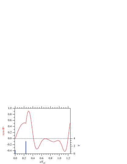
Figure 1: Resulting orientation, as expressed by $\left\langle\cos\theta\right\rangle$, for the optimal 2-kick solution, along with the amplitudes of the kicks.

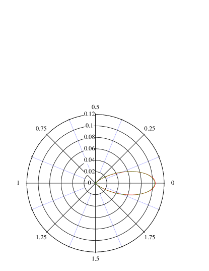
Figure 2: Polar plot of the angular distribution reached at the maximum of orientation, $t=0.3042T_{\mathrm{rot}}$ (solid line) compared with that of the target state (dotted line).

IV Conclusion

In conclusion, using evolutionary strategies, we found the optimal way to kick a molecule with short HCPs in order to reach a target state corresponding to an oriented molecule. The solution turns out to be very efficient, allowing to reach the target state (within 1%) with only two pulses, instead of the approximately 15 pulses of the previous mathematically built (but not unique) strategy of Ref. Sugny et al. (2004a) for the same system. This advocates for great experimental feasibility and, even more importantly, it points out the broad interest of the overall methodology. As has been already shown, the mathematically clear depiction of a quantum target state in a finite dimensional subspace can be conducted for a large class of observables (some examples in comparing systems interacting with a thermal baths or other dissipative environments are provided in Ref. Sugny et al. ). Once the target state is defined, ES can be successfully run with a simple criterion of maximum projection on the target state referring as a basic mechanism to a train of kicks. The only parameters to be optimized are the time delays and amplitudes. A small number of such kicks, reachable within modest experimental environment, allow for a remarkably efficient and persistent control.