Live and Dead Nodes

Abstract

In this paper, we explore the consequences of a distinction between ‘live’ and ‘dead’ network nodes; ‘live’ nodes are able to acquire new links whereas ‘dead’ nodes are static. We develop an analytically soluble growing network model incorporating this distinction and show that it can provide a quantitative description of the empirical network composed of citations and references (in- and out-links) between papers (nodes) in the SPIRES database of scientific papers in high energy physics. We also demonstrate that the death mechanism alone can result in power law degree distributions for the resulting network.

1 Introduction

The study and modeling of complex networks has expanded rapidly in the new millennium and is now firmly established as a science in its own right [Watts, 1999, Albert & Barabási, 2002, Dorogovtsev & Mendes, 2002, Newman, 2003]. One of the oldest examples of a large complex network is the network of citations and references (in- and out-links) between scientific papers (nodes) [de Solla Price, 1965, Redner, 1998, Lehmann et al., 2003, Lehmann et al., 2005, Redner, 2004]. A very successful model describing networks with power-law degree distributions is based on the notion of preferential attachment. The principles underlying this model were first introduced by Simon [Simon, 1957], applied to citation networks by de Solla Price [de Solla Price, 1976], and independently rediscovered by Barabási and Albert [Barabási & Albert, 1999]. Various modifications of the preferential attachment model have appeared more recently. In the present context, the key papers on preferential attachment are [Lehmann et al., 2003, Lehmann et al., 2005, Krapivsky et al., 2000, Krapivsky & Redner, 2001, Klemm & Eguíluz, 2002]. Simplicity is both the primary strength and the primary weakness of the preferential attachment model. For example, preferential attachment models tend to assume that networks are homogeneous. When networks have significant and identifiable inhomogeneities (as is the case for the citation network), the data can require augmentation of the preferential attachment model to account for them.

The primary conclusion of Ref. [Lehmann et al., 2003] is that the majority of nodes in a citation network ‘die’ after a short time, never to be cited again. A small population of papers remains ‘alive’ and continues to be cited many years after publication. In Ref. [Lehmann et al., 2005] it was established that this distinction between live and dead papers is an important inhomogeneity in the citation network that is not accounted for by the simple preferential attachment model. Interestingly, a similar distinction between live and dead nodes was recently independently suggested by [Redner, 2004]. In this paper, we will explore how the distinction between live and dead papers manifests itself in network models and thus suggest an extension of the preferential attachment model.

2 The SPIRES data

The work in this paper is based on data obtained from the SPIRES database of papers in high energy physics. More specifically, our dataset is the network of all citable papers from the theory subfield, ultimo October 2003. After filtering out all papers for which no information of time of publication is available and removing all references to papers not in SPIRES, a final network of $275\,665$ nodes and $3\,434\,175$ edges remains.

Above we described a dead node as one that no longer receives citations, but how does one define a dead node in real data? We have tested several definitions, and the results are qualitatively independent of the definition chosen. Therefore, we can simply define live papers as papers cited in 2003. While we acknowledge the existence of papers that receive citations after a long dormant period, such cases are rare and do not affect the large scale statistics. In Figure 2, the (normalized) degree distributions of live and dead papers in the SPIRES data are plotted, and it is clear that the two distributions differ significantly. Having isolated the dead papers, we are not only able to plot them; we can also determine the empirical ratio of live to dead papers as a function of the number of citations per paper, $k$. In Figure 1 this ratio is displayed with $k$

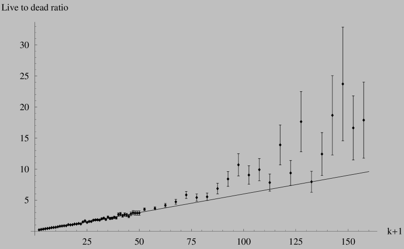
Figure 1: Displayed above is ratio of live to dead papers as a function of $k$. Error bars are calculated from square roots of the citation counts in each bin. Also, a straight line is present to illustrate the linear relationship between the live and dead populations for low values of $k$.

ranging from $1$ to $150$ (Papers with zero citations are dead by definition.) Over most of this range, the data is well described by a straight line. Note that the data for dead papers with high citation counts is very sparse. For example, only $0.15\%$ of the dead papers have more than 100 citations, so the statistics beyond this point are highly unreliable. More generally, a linear plot of the ratio of live to dead papers provides a pessimistic representation of the data. We therefore conclude that the ratio of dead to live papers is relatively well described by the simple form $1/(k+1)$ for all but the largest values of $k$, for which the number of dead papers is overestimated by a factor of two to three. In the following section, we will make use of this relation to extend the preferential attachment model to include dead nodes.

3 The Model

The basic elements of the preferential attachment model are growth and preferential attachment [Barabási & Albert, 1999]. The simplest model starts out with a number of initial nodes and at each update, a new node is added to the database. Each new node has $m$ out-links that connect to the nodes already in the database. Each new node enters with $k=0$ real in-links. This is the growth element of the model. Note that, since we have chosen to eliminate all references to papers not in SPIRES from the dataset, there is a sum rule such that the average number of citations per paper is also $m$. Preferential attachment enters the model through the assumption that the probability for a given node already in the database to receive one of the $m$ new in-links is proportional to its current number of in-links. In order for the newest nodes (with $k=0$ in-links) to be able to begin attracting new citations, we load each node into the database with $k_{0}=1$ ‘ghost’ in-links that can be subtracted after running the model. The probability of acquiring new citations is proportional to the total number of in-links, both real and ghost in-links.

One of the simplest ways to implement this simple incarnation of the preferential attachment model described above is to regard $k_{0}$ as a free parameter. This allows us to estimate when the effects of preferential attachment become important. Since there is no a priori reason why a paper with 2 citations (in-links) should have a significant advantage over a paper with 1 citation, it is preferable to let the data decide. Thus, in our model, the probability that a live paper with $k$ citations acquires a new citation at each time step is proportional to $k+k_{0}$ with $k_{0}>0$. Also, note that we can think of the displacement $k_{0}$ as a way to interpolate between full preferential attachment ($k_{0}=1$) and no preferential attachment ($k_{0}\to\infty$).

The significant extension of the simple model to be considered here is that, in our model, each paper has some probability of dying at every time step. From Section 2, we have a very good idea of what this probability should be: Figure 1 shows us that for a paper with $k$ citations, this probability is proportional to $1/(k+1)$ to a reasonable approximation. With this qualitative description of the model in hand, we proceed to its solution.

4 Rate Equations

One very powerful method for solving preferential attachment network models is the rate equation approach, introduced in the context of networks by [Krapivsky et al., 2000]. Let $L_{k}$ and $D_{k}$ be the respective probabilities of finding a live or a dead paper with $k$ real citations. As explained above, we load each paper into the database with $k=0$ real citations and $m$ references. The rate equations become

$$L_{k} = m(\lambda_{k-1}L_{k-1}-\lambda_{k}L_{k})-\eta_{k}L_{k}+\delta_{k,0}$$ (1)

$$D_{k} = \eta_{k}L_{k},$$ (2)

where $\lambda_{k}$ and $\eta_{k}$ are rate constants. Since every paper has a finite number of citations, the probabilities $L_{k}$ and $D_{k}$ become exactly zero for sufficiently large $k$; we also define $L_{k}$ to be zero for $k<0$. In this way, all sums can run from $k=0$ to infinity. These equations trivially satisfy the normalization condition

$$\sum_{k}(L_{k}+D_{k})=1,$$ (3)

for any choice of $\eta_{k}$ and $\lambda_{k}$. However, we also demand that the mean number of references is equal to the mean number of papers

$$\sum_{k}k(L_{k}+D_{k})=m.$$ (4)

This constraint must be imposed by an overall scaling of $\eta_{k}$ and $\lambda_{k}$. The model described in Section 3 corresponds to a choice of $\eta_{k}$ and $\lambda_{k}$, where

$$m\lambda_{k}=a(k+k_{0})$$ (5)

is the preferential attachment term and

$$\eta_{k}=\frac{b}{k+1}$$ (6)

corresponds to the previously described death mechanism. We insert Equations (5) and (6) into Equation (1) and perform the recursion to find

$$L_{k}=\frac{\Gamma(k+2)}{ak_{1}k_{2}}\frac{\Gamma(k+k_{0})}{\Gamma(k_{0})}\frac{\Gamma(1-k_{1})}{\Gamma(k-k_{1}+1)}\frac{\Gamma(1-k_{2})}{\Gamma(k-k_{2}+1)},$$ (7)

and of course $D_{k}=bL_{k}/(k+1)$. The two new constants, $k_{1}$ and $k_{2}$ are solutions to the quadratic equation

$$(a(k+k_{0})+1)(k+1)+b=0$$ (8)

as a function of $k$.

5 The $k_{0}\to\infty$ Limit

Before moving on, let us explore the limit where $k_{0}\to\infty$ and preferential attachment is turned off. In this regime, the network is, of course, completely dominated by the death mechanism. We can either obtain this limit by again solving Equations (1) and (2) with $\lambda_{k}=constant$ and $\eta_{k}=b/(k+1)$, or we can make the more elegant replacement $\alpha=ak_{0}$ in Equation (7), and then take the limit $k_{0}\to\infty$ for fixed $\alpha$. The two approaches are equivalent. We find

$$L_{k}=\frac{1}{\alpha}\left(\frac{\alpha}{1+\alpha}\right)^{k+1}\frac{(\frac{b}{1+\alpha})!(k+1)!}{(\frac{b}{1+\alpha}+k+1)!},$$ (9)

and the $D_{k}$ are still simply $bL_{k}/(k+1)$. With this expression for $L_{k}$, let us consider the limit of $\alpha\to\infty$ and $b\to\infty$ with the ratio $r=b/(\alpha+1)\approx b/\alpha$ fixed. In this limit, it is tempting to replace the term $\alpha/(\alpha+1)$ by one. In this case, the use of identities, such as

$$\sum^{\infty}_{k=1}\frac{k!}{(k+r)!}=\frac{1}{(1-r)r!}$$ (10)

enable us to compute the fraction of dead papers $f$, and the average numbers of citations for live and dead papers. The results are simply

$$1-f = \frac{1}{\alpha-1}$$ (11)

$$m_{L} = \frac{2}{r-2}$$ (12)

$$m_{D} = \frac{1}{r-1},$$ (13)

and the average number of citations for all papers is evidently $m=(1-f)m_{L}+fm_{D}$. The fraction of dead papers is $f\to 1-\mathcal{O}(1/b)$ and the average number of citations for all papers approaches $m_{D}$.

The most important result, however, is that in this limit we find that

$$L_{k}\sim\frac{1}{k^{r}}\quad\textrm{and}\quad D_{k}\sim\frac{b}{k^{r+1}},$$ (14)

where we assume that $k>r$. Thus, we see that power law distributions for both live and dead papers emerge naturally in the limit of $f\to 1$. In the literature, power laws in the degree distributions of networks are often regarded as an indication that preferential attachment has played an essential part in the generation of the network in question. It is thus of considerable interest to see an alternative and quite different way of obtaining them.

6 The Full Model

Let us now return to the full model and see how it compares to the data from SPIRES. With all zero cited papers in the dead category, the data yields the following average values: $m_{L}=34.1$, $m_{D}=4.5$ and $m=12.8$. The fraction of live papers is $f=27.0\%$. With an rms. error of only 21%, we can do a least squares fit of $L_{k}$ to the distribution of live papers with parameters $k_{0}=65.6$, $a=0.436$, and $b=12.4$. Although only the live data (the squares in Figure 2) is fitted, the agreement with the

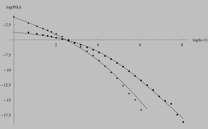
Figure 2: Log-log plots of the normalized degree distributions of live and dead papers. The filled squares represent the live data and the stars represent the dead data. Both lines are the result of a fit to the live data (filled squares) alone.

empirical data in Figures 2 and 3 is

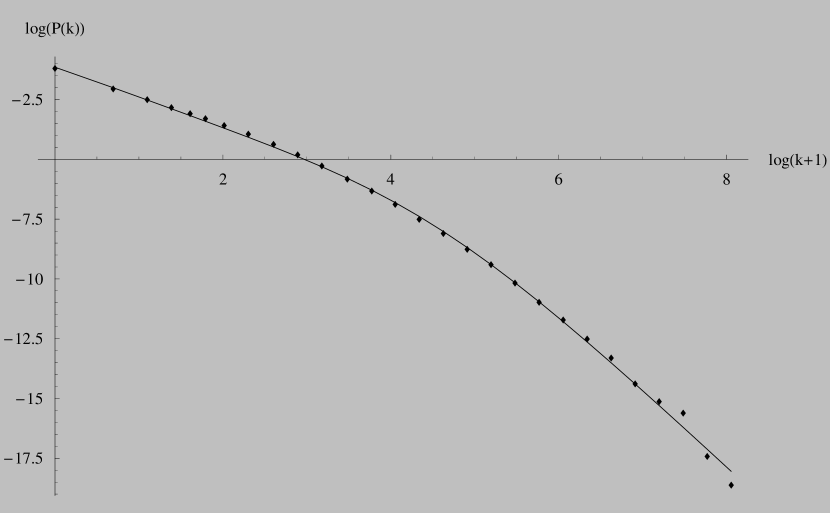
Figure 3: A log-log plot of the normalized degree distribution of all papers (live plus dead). The points are the data; the fit (solid line) is derived from the fit to the live papers (filled squares) in Figure 2.

quite striking.

From the model parameters $k_{0},a,b$, we can calculate mean citation numbers for the fit of $32.9$, $4.25$, and $12.8$ for the live, dead, and total population respectively; the fraction of live papers is found to be $29.8\%$. More interestingly, we learn from the fit that $7.5\%$ of the papers with 0 citations are actually alive. If we assign this fraction of the zero-cited papers to the live population, we find the following corrected values for the average values $31.5$, $4.6$ and $12.5$ for the live, dead, and total population respectively; the fraction of live papers is adjusted to become $29.2\%$. Again, this is a striking agreement with the data. There is so little strain in the fit that we could have determined the model parameters from the empirical values of $m_{L}$, $m_{D}$, and $f$. Doing this yields only small changes in the model parameters and results in a description of comparable quality!

Figure 2 reveals that fitting to the live distributions, results in systematic errors for high values of $k$ when we extend the fit to describe the dead papers, but this is not surprising. Recall the similarly systematic deviations from the straight line seen in Figure 1. This figure also explains why the fit to the total distribution shows no deviations from the fit for high $k$-values even though the total fit includes both live and dead papers—live papers dominate the total distribution in this regime. The obvious way to fix this problem is via a small modification of the $\eta_{k}$. In summary, the full model is able to fit the distributions of both live and dead papers with remarkable accuracy.

One drawback, with regard to the full solution is the relatively impenetrable expression for $L_{k}$ in Equation (7)—associating any kind of intuition to the conglomerate of gamma-functions presented there can be difficult. Let us therefore demonstrate that $L_{k}$ can be well approximated by a two power law structure. We begin by noting that, in the limit of large $k_{0}$ (as it is the case here), the values of $k_{1}$ and $k_{2}$ are simply

$$k_{1} = -\frac{1}{a}+\frac{b}{ak_{0}}-k0$$ (15)

$$k_{2} = -1-\frac{b}{ak0}.$$ (16)

Now, let us write out only the $k$-dependent terms in Equation (7) and assign the remaining terms to a constant, $C$

$$L_{k} = C\frac{(k+k_{0}-1)!}{(k-k_{1})!}\frac{(k+1)!}{(k-k_{2})!}$$ (17)

$$\approx C\frac{1}{(k+k_{0}-1)^{1-k_{0}-k_{1}}}\frac{1}{(k+1)^{-(1+k_{2})}}$$ (18)

$$\approx C\frac{1}{(k+k_{0}-1)^{1+\frac{1}{a}-\frac{b}{ak_{0}}}}\frac{1}{(k+1)^{\frac{b}{ak_{0}}}},$$ (19)

In Equation (18), we have utilized the fact that

$$\frac{(x+s)!}{x!}\approx x^{s}$$ (20)

when $x\to\infty$, and in Equation (19) we have inserted the asymptotic forms of $k_{1}$ and $k_{2}$, from Equations (15) and (16).

This expression for $L_{k}$ in Equation (19) is only valid for large $k$ and $k_{0}$, but it proves to be remarkably accurate even for smaller values of $k$. With the asymptotic forms of $k_{1}$ and $k_{2}$ inserted, we can explicitly see that the first power law is largely due to preferential attachment and that the second power law is exclusively due to the death mechanism. The form for very large $k$ is unaltered by the parameter $b$. This is not surprising, since there is a low probability for highly cited papers to die. We see that the primary role of the death mechanism in the full model is to add a little extra structure to the $L_{k}$ for small $k$.

7 Conclusions

Compelled by a significant inhomogeneity in the data, we have created a model that provides an excellent description of the SPIRES database. It is obvious that the death mechanism $(b\neq 0)$ is essential for describing the live and dead populations separately, but less clear that it is indispensable when it comes to the total data. Fitting the total distribution with a preferential attachment only model $(b=0)$ results in $a=0.528$ and $k_{0}=13.22$ and with a rms. fractional error of $33.6\%$. This fit displays systematic deviations from the data, but considering that the fit ignores important correlations in the dataset, the overall quality is rather high. The important lesson to learn from the work in this paper, is that even a high quality fit to the global network distributions is not necessarily an indication of the absence of additional correlations in the data.

The most significant difference between the full live-dead model and the model described above is expressed in the value of the parameter $k_{0}$. The value of this parameter changes by a factor of approximately 5, from $65.6$ to $13.2$. It strikes us as natural that preferential attachment will not be important until a paper is sufficiently visible for authors to cite it without reading it. We thus believe that $k_{0}\approx 66$ is a more intuitively appealing value for the onset of preferential attachment. However, independent of which value of the $k_{0}$ parameter one prefers, the comparison of these two models clearly demonstrates the danger of assigning physical meaning to even the most physically motivated parameters if a network contains unidentified correlations or if known correlations are neglected in the modeling process. Specifically, it would be ill advised to draw strong conclusions about the onset of preferential attachment if the death mechanism is not included in the model making.

In summary, the live and dead papers in the SPIRES database constitute distributions with significantly different statistical properties. We have constructed a model which includes modified preferential attachment and the death of nodes. This model is quantitatively successful in describing the citation distributions for live and dead papers. The resulting model has also been shown to produce a two power law structure. This structure provides an appealing link to the work in [Lehmann et al., 2003], where a two power law structure was adopted to characterize the form of the SPIRES data without any theoretical support. Finally, we have been shown that even in the absence of preferential attachment, the death mechanism alone can result in power laws. Since many real world networks have a large number of inactive nodes and only a small fraction of active nodes, we are confident that this mechanism will find more general use.

References

- Albert & Barabási, 2002 Albert, R. and A.-L. Barabási (2002), Statistical mechanics of complex networks. Reviews of modern physics, 74, 47.
- Barabási & Albert, 1999 Barabási, A.-L. and R. Albert (1999), Emergence of scaling in random networks. Science, 286, 509.
- de Solla Price, 1965 de Solla Price, D. (1965), Networks of Scientific Papers. Science, 149, 510–515.
- de Solla Price, 1976 de Solla Price, D. (1976), A General Theory of Bibliometric and Other Cumulative Advantage Processes. Journal of the American Society for Information Science, 27, 292.
- Dorogovtsev & Mendes, 2002 Dorogovtsev, S. N. and J. F. F. Mendes (2002), Evolution of networks. Advances in Physics, 51, 1079.
- Klemm & Eguíluz, 2002 Klemm, K. and V. M. Eguíluz (2002), Highly Clustered Scale-Free Networks. Physical Review E, 65, 036123.
- Krapivsky & Redner, 2001 Krapivsky, P. L., and S. Redner (2001), Organization of Growing Random Networks. Physical Review E, 63, 066123.
- Krapivsky et al., 2000 Krapivsky, P. L., S. Redner and F. Leyvraz (2000), Connectivity of Growing Random Networks. Physical Review Letters, 85(21), 4629.
- Lehmann et al., 2003 Lehmann, S., B. E. Lautrup and A. D. Jackson (2003), Citation networks in high energy physics. Physical Review E, 68.
- Lehmann et al., 2005 Lehmann, S., A. D. Jackson and B. E. Lautrup (2005), Life, Death, and Preferential Attachment. Europhysics Letters, 69, 298.
- Newman, 2003 Newman, M. E. J. (2003), The structure and function of complex networks. SIAM Review, 45, 167.
- Redner, 1998 Redner, S. (1998). How popular is your paper? An emperical study of the citation distribution. European Physics Journal B, 4, 131–4.
- Redner, 2004 Redner, S. (2004), Citation Statistics From More Than a Century of Physical Review. physics/0407137.
- Simon, 1957 Simon, H. A. (1957), Models of Man. New York: Wiley.
- Watts, 1999 Watts, D. J. (1999), Small Worlds. Princeton: Princeton University Press.