Analyzing money distributions in ‘ideal gas’ models of markets

We analyze an ideal gas like models of a trading market. We propose a new fit for the money distribution in the fixed or uniform saving market. For the market with quenched random saving factors for its agents we show that the steady state income ($m$) distribution $P(m)$ in the model has a power law tail with Pareto index $\nu$ exactly equal to unity, confirming the earlier numerical studies on this model. We analyze the distribution of mutual money difference and also develop a master equation for the time development of $P(m)$. Precise solutions are then obtained in some special cases.

1 Introduction

The distribution of wealth among individuals in an economy has been an important area of research in economics, for more than a hundred years. Pareto Pareto:1897 first quantified the high-end of the income distribution in a society and found it to follow a power-law $P(m)\sim m^{-(1+\nu)}$, where $P$ gives the normalized number of people with income $m$, and the exponent $\nu$, called the Pareto index, was found to have a value between 1 and 3.

Considerable investigations with real data during the last ten years revealed that the tail of the income distribution indeed follows the above mentioned behavior and the value of the Pareto index $\nu$ is generally seen to vary between 1 and 2.5 Oliveira:1999 ; realdatag ; realdataln ; Sitabhra:2005 . It is also known that typically less than $10\%$ of the population in any country possesses about $40\%$ of the total wealth of that country and they follow the above law. The rest of the low income population, in fact the majority ($90\%$ or more), follow a different distribution which is debated to be either Gibbs realdatag ; marjit or log-normal realdataln .

Much work has been done recently on models of markets, where economic (trading) activity is analogous to some scattering process marjit ; Chakraborti:2000 ; Chatterjee:2004 ; Chatterjee:2003 ; Chakrabarti:2004 ; othermodels ; Slanina:2004 . We put our attention to models where introducing a saving factor for the agents, a wealth distribution similar to that in the real economy can be obtained Chakraborti:2000 ; Chatterjee:2004 . Savings do play an important role in determining the nature of the wealth distribution in an economy and this has already been observed in some recent investigations Willis:2004 . Two variants of the model have been of recent interest; namely, where the agents have the same fixed saving factor Chakraborti:2000 , and where the agents have a quenched random distribution of saving factors Chatterjee:2004 . While the former has been understood to a certain extent (see e.g, Das:2003 ; Patriarca:2004 ), and argued to resemble a gamma distribution Patriarca:2004 , attempts to analyze the latter model are still incomplete (see however, Repetowicz:2004 ). Further numerical studies Ding:2003 of time correlations in the model seem to indicate even more intriguing features of the model. In this article, we intend to study both the market models with savings, analyzing the money difference in the models.

2 The model

The market consists of $N$ (fixed) agents, each having money $m_{i}(t)$ at time $t$ ($i=1,2,\ldots,N$). The total money $M$ ($=\sum_{i}^{N}m_{i}(t)$) in the market is also fixed. Each agent $i$ has a saving factor $\lambda_{i}$ ($0\leq\lambda_{i}<1$) such that in any trading (considered as a scattering) the agent saves a fraction $\lambda_{i}$ of its money $m_{i}(t)$ at that time and offers the rest $(1-\lambda_{i})m_{i}(t)$ for random trading. We assume each trading to be a two-body (scattering) process. The evolution of money in such a trading can be written as:

$$m_{i}(t+1)=\lambda_{i}m_{i}(t)+\epsilon_{ij}\left[(1-\lambda_{i})m_{i}(t)+(1-\lambda_{j})m_{j}(t)\right],$$ (1)

$$m_{j}(t+1)=\lambda_{j}m_{j}(t)+(1-\epsilon_{ij})\left[(1-\lambda_{i})m_{i}(t)+(1-\lambda_{j})m_{j}(t)\right]$$ (2)

where each $m_{i}\geq 0$ and $\epsilon_{ij}$ is a random fraction ($0\leq\epsilon\leq 1$). In the fixed savings market $\lambda_{i}=\lambda_{j}$ for all $i$ and $j$, while in the distributed savings market $\lambda_{i}\neq\lambda_{j}$ with $0\leq\lambda_{i},\lambda_{j}<1$.

3 Numerical observations

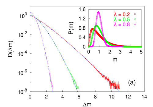
Figure 1: $D(\Delta)$ in the fixed or uniform savings market, for $\lambda=0.2,0.5,0.8$ (right to left) and their fitting curves: $D(\Delta)\sim\exp(-\Delta^{1+\lambda}/T^{\prime})$; the corresponding $P(m)$ the inset.

In addition to what have already been reported in Ref. Chatterjee:2004 ; Chatterjee:2003 ; Chakrabarti:2004 for the model, we observe that, for the market with fixed or uniform saving factor $\lambda$, a fit to Gamma distribution Patriarca:2004 ,

$$P(m)\sim m^{\eta}\exp(-m/T),\quad\eta=\frac{3\lambda}{1-\lambda}$$ (3)

is found to be better than a log-normal distribution. However, our observation regarding the distribution $D(\Delta)$ of difference $\Delta\equiv|\Delta m|$ of money between any two agents in the market (see Fig. 1a) suggests a different form:

$$P(m)\sim m^{\delta}\exp(-m^{\kappa}/T^{\prime});\quad\kappa=1+\lambda.$$ (4)

In fact, we have checked, the steady state (numerical) results for $P(m)$ asymptotically fits even better to (3), rather than to (4).

With heterogeneous saving propensity of the agents with fractions $\lambda$ distributed (quenched) widely ($0\leq\lambda<1$), where the market settles to a critical Pareto distribution $P(m)\sim m^{-(1+\nu)}$ with $\nu\simeq 1$ Chatterjee:2004 , the money difference behaves as $D(\Delta m)\sim(\Delta m)^{-(1+\gamma)}$ with $\gamma\simeq 1$. In fact, this behavior is invariant even if we set $\epsilon_{ij}=1/2$ Chatterjee:2005 . This can be justified by the earlier numerical observation Chakraborti:2000 ; Chatterjee:2004 for fixed $\lambda$ market ($\lambda_{i}=\lambda$ for all $i$) that in the steady state, criticality occurs as $\lambda\to 1$ where of course the dynamics becomes extremely slow. In other words, after the steady state is realized, the third term containing $\epsilon=1/2$ becomes unimportant for the critical behavior. We therefore concentrate on this case in this paper.

4 Analysis of money difference

In the process as considered above, the total money $(m_{i}+m_{j})$ of the pair of agents $i$ and $j$ remains constant, while the difference $\Delta m_{ij}$ evolves for $\epsilon=1/2$ as

$$(\Delta m_{ij})_{t+1}=\alpha_{ij}(\Delta m_{ij})_{t}+\beta_{ij}(m_{i}+m_{j})_{t},$$ (5)

where $\alpha_{ij}=\frac{1}{2}(\lambda_{i}+\lambda_{j})$ and $\beta_{ij}=\frac{1}{2}(\lambda_{i}-\lambda_{j})$. As such, $0\leq\alpha<1$ and $-\frac{1}{2}<\beta<\frac{1}{2}$. The steady state probability distribution $D(\Delta)$ can be written as (cf. Chatterjee:2005 ):

$$D(\Delta) = \int d\Delta^{\prime}\;D(\Delta^{\prime})\;\langle\delta(\Delta-(\alpha+\beta)\Delta^{\prime})+\delta(\Delta-(\alpha-\beta)\Delta^{\prime})\rangle$$ (6)

$$= 2\langle\left(\frac{1}{\lambda}\right)\;D\left(\frac{\Delta}{\lambda}\right)\rangle,$$

where we have used the symmetry of the $\beta$ distribution and the relation $\alpha_{ij}+\beta_{ij}=\lambda_{i}$, and have suppressed labels $i$, $j$. Here $\langle\ldots\rangle$ denote average over $\lambda$ distribution in the market. Taking now a uniform random distribution of the saving factor $\lambda$, $\rho(\lambda)=1$ for $0\leq\lambda<1$, and assuming $D(\Delta)\sim\Delta^{-(1+\gamma)}$ for large $\Delta$, we get

$$1=2\int d\lambda\;\lambda^{\gamma}=2(1+\gamma)^{-1},$$ (7)

giving $\gamma=1$. No other value fits the above equation. This also indicates that the money distribution $P(m)$ in the market also follows a similar power law variation, $P(m)\sim m^{-(1+\nu)}$ and $\nu=\gamma$.

5 Master equation approach

We also develop a Boltzmann-like master equation for the time development of $P(m,t)$, the probability distribution of money in the market Chatterjee:2005 . We again consider the case $\epsilon_{ij}=\frac{1}{2}$ in (1) and (2) and rewrite them as

$$\left(\begin{array}[]{c}m_{i}\\ m_{j}\end{array}\right)_{t+1}=\mathcal{A}\left(\begin{array}[]{c}m_{i}\\ m_{j}\end{array}\right)_{t}{\rm where}\;\;\;\mathcal{A}=\left(\begin{array}[]{cc}\mu_{i}^{+}&\mu_{j}^{-}\\ \mu_{i}^{-}&\mu_{j}^{+}\end{array}\right);\quad\mu^{\pm}=\frac{1}{2}(1\pm\lambda).$$ (8)

Collecting the contributions from terms scattering in and subtracting those scattering out, we can write the master equation for $P(m,t)$ as

$$\frac{\partial P(m,t)}{\partial t}+P(m,t)=\langle\int dm_{i}\int dm_{j}\;P(m_{i},t)P(m_{j},t)\;\delta(\mu_{i}^{+}m_{i}+\mu_{j}^{-}m_{j}-m)\rangle,$$ (9)

which in the steady state gives

$$P(m)=\langle\int dm_{i}\int dm_{j}\;P(m_{i})P(m_{j})\;\delta(\mu_{i}^{+}m_{i}+\mu_{j}^{-}m_{j}-m)\rangle.$$ (10)

Assuming, $P(m)\sim m^{-(1+\nu)}$ for $m\rightarrow\infty$, we get Chatterjee:2005

$$1=\langle(\mu^{+})^{\nu}+(\mu^{-})^{\nu}\rangle\equiv\int\int d\mu^{+}d\mu^{-}p(\mu^{+})q(\mu^{-})\left[(\mu^{+})^{\nu}+(\mu^{-})^{\nu}\right].$$ (11)

Considering now the dominant terms ($\propto x^{-r}$ for $r>0$, or $\propto\ln(1/x)$ for $r=0$) in the $x\to 0$ limit of the integral $\int_{0}^{\infty}m^{(\nu+r)}P(m)\exp(-mx)dm$, we get from eqn. (11), after integrations, $1=2/(\nu+1)$, giving finally $\nu=1$.

6 Summary

We consider the ideal-gas-like trading markets where each agent is identified with a gas molecule and each trading as an elastic or money-conserving (two-body) collision Chakraborti:2000 ; Chatterjee:2004 ; Chatterjee:2003 ; Chakrabarti:2004 . Unlike in a gas, we introduce a saving factor $\lambda$ for each agents. Our model, without savings ($\lambda=0$), obviously yield a Gibbs law for the steady-state money distribution. Our numerical results for uniform saving factor suggests the equilibrium distribution $P(m)$ to be somewhat different from the Gamma distribution reported earlier Patriarca:2004 .

For widely distributed (quenched) saving factor $\lambda$, numerical studies showed Chatterjee:2004 ; Chatterjee:2003 ; Chakrabarti:2004 that the steady state income distribution $P(m)$ in the market has a power-law tail $P(m)\sim m^{-(1+\nu)}$ for large income limit, where $\nu\simeq 1.0$, and this observation has been confirmed in several later numerical studies as well Repetowicz:2004 ; Ding:2003 . It has been noted from these numerical simulation studies that the large income group people usually have larger saving factors Chatterjee:2004 . This, in fact, compares well with observations in real markets Willis:2004 ; Dynan:2004 . The time correlations induced by the random saving factor also has an interesting power-law behavior Ding:2003 . A master equation for $P(m,t)$, as in (9), for the original case (eqns. (1) and (2)) was first formulated for fixed $\lambda$ ($\lambda_{i}$ same for all $i$), in Das:2003 and solved numerically. Later, a generalized master equation for the same, where $\lambda$ is distributed, was formulated and solved in Repetowicz:2004 and Chatterjee:2005 . We show here that our analytic study (see Chatterjee:2005 for details) clearly support the power-law for $P(m)$ with the exponent value $\nu=1$ universally, as observed numerically earlier Chatterjee:2004 ; Chatterjee:2003 ; Chakrabarti:2004 .

7 Acknowledgments

BKC is grateful to the INSA-Royal Society Exchange Programme for financial support to visit the Rudolf Peierls Centre for Theoretical Physics, Oxford University, UK and RBS acknowledges EPSRC support under the grants GR/R83712/01 and GR/M04426 for this work and wishes to thank the Saha Institute of Nuclear Physics for hospitality during a related visit to Kolkata, India.

References

- (1) Pareto V (1897) Cours d’economie Politique. F. Rouge, Lausanne
- (2) Moss de Oliveira S, de Oliveira PMC, Stauffer D (1999) Evolution, Money, War and Computers. B. G. Tuebner, Stuttgart, Leipzig
- (3) Levy M, Solomon S (1997) Physica A 242:90-94; Drăgulescu AA, Yakovenko VM (2001) Physica A 299:213; Aoyama H, Souma W, Fujiwara Y (2003) Physica A 324:352
- (4) Di Matteo T, Aste T, Hyde ST (2003) cond-mat/0310544; Clementi F, Gallegati M (2004) cond-mat/0408067
- (5) Sinha S (2005) cond-mat/0502166
- (6) Chakrabarti BK, Marjit S (1995) Ind. J. Phys. B 69:681; Ispolatov S, Krapivsky PL, Redner S (1998) Eur. Phys. J. B 2:267; Drăgulescu AA, Yakovenko VM (2000) Eur. Phys. J. B 17:723
- (7) Chakraborti A, Chakrabarti BK (2000) Eur. Phys. J. B 17:167
- (8) Chatterjee A, Chakrabarti BK, Manna SS (2004) Physica A 335:155
- (9) Chatterjee A, Chakrabarti BK; Manna SS (2003) Phys. Scr. T 106:36
- (10) Chakrabarti BK, Chatterjee A (2004) in Application of Econophysics, Proc. 2nd Nikkei Econophys. Symp., ed. Takayasu H, Springer, Tokyo, pp. 280-285
- (11) Hayes B (2002) Am. Scientist (Sept-Oct) 90:400; Sinha S (2003) Phys. Scr. T 106:59; Ferrero JC (2004) Physica A 341:575; Iglesias JR, Gonçalves S, Abramson G, Vega JL (2004) Physica A 342:186; Scafetta N, Picozzi S, West BJ (2004) Physica D 193:338
- (12) Slanina F (2004) Phys. Rev. E 69:046102
- (13) Willis G, Mimkes J (2004) cond-mat/0406694
- (14) Das A, Yarlagadda S (2003) Phys. Scr. T 106:39
- (15) Patriarca M, Chakraborti A, Kaski K (2004) Phys. Rev. E 70:016104
- (16) Repetowicz P, Hutzler S, Richmond P (2004) cond-mat/0407770
- (17) Ding N, Xi N, Wang Y (2003) Eur. Phys. J. B 36:149
- (18) Chatterjee A, Chakrabarti BK, Stinchcombe RB (2005) cond-mat/0501413
- (19) Dynan KE, Skinner J, Zeldes SP (2004) J. Pol. Econ. 112:397.