Free-Space Antenna Field/Pattern Retrieval
in Reverberation Environments

Abstract

Simple algorithms for retrieving free-space antenna field or directivity patterns from complex (field) or real (intensity) measurements taken in ideal reverberation environments are introduced and discussed.

I Introduction

Antenna measurements are usually performed under simulated free-space conditions, e.g. by placing the antenna under test (henceforth AUT) as well as the measuring probe in an open test-range or in an electromagnetic (henceforth EM) anechoic chamber [1].

Retrieving free-space antenna field and/or directivity patterns from measurements taken in any realistic (i.e., imperfect) test-range or anechoic chamber relies on the possibility of reconstructing the ray skeleton of the measured field using robust spectral estimation techniques, including, e.g., periodogram, Prony, Pisarenko, Matrix-Pencil and Gabor algorithms [2]-[5], so as to ”subtract” all environment-related reflected/diffracted fields.

The direct (free-space) field, however, cannot be unambiguously identified, unless additional assumptions are made about its relative intensity and/or phase, which do not hold true in the most general case.

A possible way to uniquely extract the free-space (direct path) field is to average over many measurements obtained by suitably changing the position of the source-probe pair with respect to the environment, while keeping the source-probe mutual distance and orientation fixed. This obviously leaves the free-space direct-path term unchanged, while affecting both the amplitudes and the phases of all environment-related reflected/diffracted fields. In the limit of a large number of measurements, one might expect that these latter would eventually average to zero. This is the rationale behind the idea of retrieving free-space antenna parameters from measurements taken in a reverberation enclosure (henceforth RE), where the chamber boundary is effectively moved through several positions by mechanical stirring, while the source-probe distance and mutual orientation is fixed.

Through the last decades reverberation enclosures earned the status of elicited EMI-EMC assessment tools [6]. On the other hand, only recently effective procedures for estimating antenna parameters, including efficiency [7], diversity-gain [8], MIMO-array channel capacity [9], and free-space radiation resistance [10], from measurements made in a reverberation chamber have been introduced by Kildal and co-workers, in a series of pioneering papers.

Here we discuss, perhaps for the first time, free-space antenna field/directivity pattern retrieval from measurements taken in a reverberation environment.

The paper is organized as follows. In Sect. II the key relevant properties of reverberation enclosure fields are summarized. In Sect. III and IV simple algorithms for retrieving free-space antenna field or directivity patterns, respectively from (complex) field or (real) intensity measurements made in a reverberation environment are discussed, including the related absolute and relative errors. The related efficiency is the subject of Sect. V, including some useful concepts on Cramer-Rao bounds. Conclusions follow under Sect. VI.

II Fields in Reverberation Environments

In the following we shall sketch and evaluate some straightforward procedures to estimate the free-space antenna field or directivity pattern from measurements made in a reverberation enclosure.

The AUT field/intensity will be sampled at a suitable number of points $P$ of the AUT-centered sphere $r\!=\!R$, corresponding to as many sampling directions. At each point $P$ we shall actually make $N$ measurements in the reverberation environment corresponding to as many different positions of the mode stirrers.

Throughout the rest of this paper we shall restrict to the simplest case where both the antenna under test and the field-probe (henceforth FP) are linearly (co)polarized, and placed in an ideal (fully-stirred) reverberation environment.

The relevant component of the complex electromagnetic (henceforth EM) field at a point $P$ can be written:

$$E(P,n)\!=\!E_{d}(P)\!+\!E_{r}(P,n),~{}~{}n\!=\!1,2,\!\dots\!,N.$$ (1)

The first term in (1) is the direct field, and is the only term which would exist in free-space; the second term is the (pure) reverberation field, whose value depends on the stirrers’ positions, and $n$ identifies the different stirrers’ positions.

According to a widely accepted model [11], for any fixed $P$, the set $\{E_{r}(P,n)|n=1,2,\dots,N\}$, can be regarded as an ensemble of identically distributed (pseudo) random variables resulting from the superposition of a large number of plane waves with uniformly distributed phases and arrival directions.

Under these ideal (but not unrealistic) assumptions the real and imaginary part of the reverberation field $E_{r}(P,n)$ will be gaussian distributed and uncorrelated, with zero averages and equal variances [13],

$$\langle\mbox{Re}^{2}E_{r}(P,n)\rangle=\langle\mbox{Im}^{2}E_{r}(P,n)\rangle=\frac{E_{0}^{2}}{2},$$ (2)

where $\langle\cdot\rangle$ denotes, more or less obviously, statistical averaging. The quantity $E_{0}^{2}$ in (2) is given by [11]:

$$E_{0}^{2}=\frac{8\pi\eta_{0}}{\lambda^{2}}~{}\Pi_{r},$$ (3)

where $\eta_{0}$ is the free-space wave impedance, $\lambda$ the wavelength, and $\Pi_{r}$ the power received by any (linearly polarized, matched) antenna placed in the reverberation enclosure, irrespective of its orientation and directivity diagram [11]. This latter is related to the total power $\Pi_{t}$ radiated into the enclosure by the AUT as follows [14] :

$$\Pi_{r}=\Xi~{}\Pi_{t},$$ (4)

where the (frequency dependent) RE calibration-parameter $\Xi$ is related to the chamber (internal) surface $\Sigma$ and wavelength $\lambda$ by [14]

$$\Xi=\frac{\lambda^{2}}{2\alpha\Sigma},$$ (5)

$\alpha$ being an average-equivalent wall absorption coefficient.

III AUT Free-Space Field Estimator

Under the made assumption where the real and imaginary part of the reverberation field $E_{r}$ are independent, zero-average gaussian random variables, it is natural to adopt the following estimator of the free-space (complex) AUT field at $P$ in terms of the (complex) fields (1):

$$\widehat{E}_{d}(P)=N^{-1}\sum_{n=1}^{N}E(P,n).$$ (6)

Equation (6) provides unbiased estimators of $\mbox{Re}[E_{d}(P)]$ and $\mbox{Im}[E_{d}(P)]$, with variances

$$VAR[\mbox{Re}\widehat{E}_{d}(P)]=VAR[\mbox{Im}\widehat{E}_{d}(P)]=\frac{E^{2}_{0}}{2N}.$$ (7)

The related absolute and relative errors are:

$$\epsilon_{abs}^{(F)}=\left\langle\left|\widehat{E}_{d}(P)-E_{d}(P)\right|^{2}\right\rangle^{1/2}=N^{-1/2}E_{0},$$ (8)

and

$$\epsilon_{rel}^{(F)}=\frac{\left\langle\left|\widehat{E}_{d}(P)-E_{d}(P)\right|^{2}\right\rangle^{1/2}}{\left|E_{d}(P)\right|}=\left(\frac{2}{N\theta}\right)^{1/2},$$ (9)

where, for later convenience, we introduced the dimensionless quantity

$$\theta(P)=\frac{2|E_{d}(P)|^{2}}{E_{0}^{2}}.$$ (10)

The r.m.s. absolute error (8) can be made as small as one wishes, in principle, by increasing $N$, and/or the chamber size (the distance between the chamber walls and the AUT-FP pair), which makes $E_{0}\propto\Sigma^{-1/2}$ smaller. Keeping the AUT-FP pair distance fixed, this will at the same time make $\theta$ larger, in view of eq. (10), thus reducing the relative error (9), when meaningful, as well. Note that this is true for both far and near-field measurements.

IV AUT Directivity Estimator

The AUT directivity can be estimated from (far field) intensity measurements made in a reverberation enclosure as follows. Let

$$I(P,n)\!=\!\mbox{Re}^{2}E(P,n)\!+\!\mbox{Im}^{2}E(P,n),~{}~{}n\!=\!1,2,\!\dots\!,N.$$ (11)

It is convenient to scale the field intensities $I(P,n)$ to the variance in (2), by letting $\xi_{n}(P)=2I(P,n)/E_{0}^{2}$, so that all the $\xi_{n}$ are (identically) distributed according to a noncentral chi-square with two degrees of freedom [15] and non-centrality parameter $\theta(P)$ given by eq. (10).

We may use the obvious far field formula:

$$|E_{d}(P)|^{2}=\frac{2\eta_{0}\Pi_{t}}{4\pi R^{2}}~{}D(P),$$ (12)

where $D(P)$ is the AUT directivity, together with eq.s (3) and (4) in eq. (10) to relate $\theta$ to the AUT directivity $D$ as follows

$$\theta=\frac{1}{8\pi^{2}\Xi(f)}\left(\frac{\lambda}{R}\right)^{2}D=:\gamma D,$$ (13)

where the dependence of $D$ and $\theta$ on the measurement point (direction) is understood and dropped for notational ease. The probability density function of the $\xi_{n}$ can be accordingly written [15]

$$f(\xi;D)=\frac{1}{2}\exp\left(-\frac{\xi+\gamma D}{2}\right)I_{0}(\sqrt{\xi\gamma D}).$$ (14)

The first two moments accordingly are:

$$\langle\xi\rangle=2+\gamma D,~{}~{}~{}VAR[\xi]=4+4\gamma D,$$ (15)

which suggest using the following (simplest, unbiased) estimator of $D$ [16]:

$$\widehat{D}=(\gamma N)^{-1}\sum_{n=1}^{N}(\xi_{n}-2),$$ (16)

for which

$$VAR[\widehat{D}]=\frac{4}{\gamma^{2}N}\left(1+\gamma D\right).$$ (17)

The absolute and relative errors of the directivity estimator (16) are thus:

$$\epsilon_{abs}^{(D)}=\sqrt{VAR[\widehat{D}]}$$ (18)

and:

$$\epsilon_{rel}^{(D)}\!=\!D^{-1}\sqrt{\left\langle\!\left(\widehat{D}\!-\!D\right)^{2}\right\rangle}\!=\!\frac{2}{\theta}\left(\frac{1+\theta}{N}\right)^{1/2}.$$ (19)

The absolute and relative (when meaningful) errors (18) and (19) can be made as small as one wishes, in principle, by increasing $N$, and/or the chamber size, so as to make $\theta$ suitably large, in view of (13).

Note that in all derivations above we made the implicit assumption of dealing with independent measurements.

The number $N$ of independent measurements needed to achieve relative errors $\sim 5\cdot 10^{-2}$ for both field and directivity measurements is shown in Fig. 1,

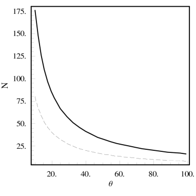
Figure 1: Number $N$ of independent measurements vs. $\theta$ needed for relative errors $\sim 5\cdot 10^{-2}$. Solid line: $\epsilon_{rel}^{(D)}$; dashed line: $\epsilon_{rel}^{(F)}$.

and is of the order of $10^{2}$ for $\theta\sim 10$. This figure is consistent with typical experimental findings [17], and also with theoretical estimates obtained from a chaos-based models of reverberation enclosures [18].

V Efficiency of Proposed Estimators

An obvious question is now whether one could do better using different estimators, other than (6) and (16).

The natural benchmark for gauging the goodness of an estimator is the well-known Cramer-Rao lower bound (henceforth CRLB) [19]. We limit ourselves here to remind a few basic definitions and properties. Let ${\mathbf{\xi}}=\{\xi_{k}|k=1,2,\dots,K\}$ a set of (real) random variables with joint probability density $f({\mathbf{\xi}};{\mathbf{X}})$, where ${\mathbf{X}}=\{X_{m}|m=1,2,\dots,M\}$ is a set of (unknown, real) parameters to be estimated. One can prove that for any estimator $\widehat{{\mathbf{X}}}$ of ${\mathbf{X}}$ such that $\langle\widehat{{\mathbf{X}}}\rangle={\mathbf{X}}$, (unbiased estimator), one has:

$${\mathbf{C}}_{\widehat{\mathbf{X}}}-{\mathbf{J}}^{-1}({\mathbf{X}})\geq 0{}$$ (20)

where ${\mathbf{C}}$ is the covariance matrix, viz.:

$$\left[{\mathbf{C}}_{\widehat{\mathbf{X}}}\right]_{hk}=\left\langle(\widehat{X}_{h}-X_{h})(\widehat{X}_{k}-X_{k})\right\rangle,$$ (21)

$$\left[{\mathbf{J}}({\mathbf{X}})\right]_{hk}=-\left\langle\frac{\partial^{2}\log{f({\mathbf{\xi}};{\mathbf{X}})}}{\partial X_{h}\partial X_{k}}\right\rangle$$ (22)

is the Fisher information matrix, the expectations are taken with respect to $f({\mathbf{\xi}};{\mathbf{X}})$, and the true value of ${\mathbf{X}}$ is used for evaluating (22). Equation (20) implies $M$ inequalities whereby the diagonal elements of ${\mathbf{C}}_{\widehat{\mathbf{X}}}$, i.e., the variances of the components of $\widehat{{\mathbf{X}}}$, are bounded from below. These are the CRLB s. An estimator for which the l.h.s. of eq. (20) is actually zero, i.e., for which the variance of each component of $\widehat{{\mathbf{X}}}$ attains its CRLB is called efficient. For the special case where the $\xi_{k}$ are independent and identically distributed, with a PDF $f(\xi;X)$ depending on a single parameter $X$, equation (20) becomes

$$VAR[\widehat{X}]\geq-\frac{1}{\displaystyle{N\left\langle\frac{\partial^{2}\log{f(\xi;X)}}{\partial X^{2}}\right\rangle}}=$$

$$=\frac{1}{\displaystyle{N\left\langle\left[\frac{\partial\log{f(\xi;X)}}{\partial X}\right]^{2}\right\rangle}}.$$ (23)

One can readily prove that the field estimator (6) is an efficient one, since the r.h.s of (7) coincides with the pertinent CRLB. The simplest directivity estimator (16), on the other hand, while not efficient, gets very close to its CRLB, as shown below.

The Cramer-Rao bound for the estimator (16), is obtained by using the following formula, which follows directly from eq. (14),

$$\frac{\partial\log f(\xi;D)}{\partial D}=-\frac{\gamma}{2}+\frac{1}{2}\frac{I_{1}\left(\sqrt{\xi\gamma D}\right)}{I_{0}\left(\sqrt{\xi\gamma D}\right)}\sqrt{\frac{\xi\gamma}{D}},$$ (24)

where $I_{0,1}(\cdot)$ are modified Bessel functions, and is [16]:

$$CRLB(D)=\frac{4}{\gamma^{2}N}\left(\frac{\Lambda}{\gamma D}-1\right)^{-1},$$ (25)

where

$$\Lambda=\left\langle\xi I_{1}^{2}\left(\sqrt{\xi\gamma D}\right)\cdot I_{0}^{-2}\left(\sqrt{\xi\gamma D}\right)\right\rangle,$$ (26)

and the expectation is taken with respect to $f(\xi;D)$.

The ratio between the CRLB (26) and the variance (17) yields the relative efficiency

$$\rho=\frac{CRLB(D)}{\mbox{VAR}[\widehat{D}]}.$$ (27)

The relative efficiency (27) of the proposed directivity estimator (16) is readily computed from eq.s (25), (26) and (17), and is independent of $N$. It is displayed in Fig. 2 vs. $\theta=\gamma D$.

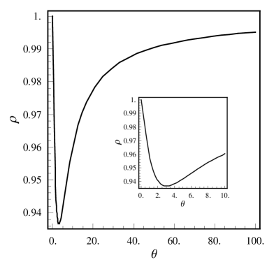
Figure 2: Directivity estimator. Relative efficiency $\rho$, eq. (27), vs. $\theta$, eq. (13).

The relative efficiency of (16) is seen to be pretty decent, being always larger than $\approx.937$.

VI Conclusions

Free-space antenna field/directivity measurements in ideal reverberation enclosures have been shortly described and evaluated. The main simplifying assumptions (linearly co-polarized AUT and FP) can be more or less easily relaxed at the expense of minor formal complications which do not alter the main conclusions. On the basis of these preliminary results, the possibility of performing cheap, simple and reliable in situ antenna measurements using, e.g., flexible conductive thin-film deployable/inflatable enclosures with air-blow stirring [20], [21] is envisaged.

References

- [1] G.E. Evans, Antenna Measurement Techniques, London:Artech House, 1990.
- [2] P.S.H. Leather and D. Parsons, ”Equalization for antenna-pattern measurements: established technique - new application”, IEEE Antennas Propagation Magazine, vol. 45, n. 2, pp. 154-161, 2003.
- [3] S. Loredo et al., ”Echo identification and cancellation techniques for antenna measurement in non-anechoic test sites”, IEEE Antennas Propagation Magazine, vol. 46, n. 1, pp. 100-107, 2004.
- [4] H. Ouibrahim, ”Prony, Pisarenko, and the matrix pencil: a unified presentation”, IEEE Transactions on Acoustic Speech and Signal Processing, vol. 37, n. 1, pp. 133-134, 1989.
- [5] B. Fourestie’ and Z. Altman, ”Gabor schemes for analyzing antenna measurements”, IEEE Transactions on Antennas and Propagation, vol. 49, n. 9, pp. 1245-1253, 2001.
- [6] M.L. Crawford, G.H. Koepke, ”Design, evaluation, and use of a reverberation chamber for performing electromagnetic susceptibility/vulnerability measurements”, Natl. Bureau of Std.s (US) Tech. Note 1092, 1986.
- [7] K. Rosengren et al., ”Characterization of antennas for mobile and wireless terminals in reverberation chambers: Improved accuracy by platform stirring”, Microwave and Optical Technology Letters, vol. 30, n. 6, pp. 391-397, 2001.
- [8] P.S. Kildal et al. ”Definition of effective diversity gain and how to measure it in a reverberation chamber”, Microwave and Optical Technology Letters, vol. 34, n. 1, pp. 56-59, 2002.
- [9] K. Rosengren et al., ”Multipath characterization of antennas for MIMO systems in reverberation chamber, including effects of coupling and efficiency”, IEEE Antennas and Propagation Society Symposium 2004, vol. 2, pp. 1712 - 1715.
- [10] P.S. Kildal et al., ”Measurement of free-space impedances of small antennas in reverberation chambers”, Microwave and Optical Technology Letters, vol. 32, n. 2, pp. 112-115, 2002.
- [11] D. A. Hill, ”Plane wave integral representation for fields in reverberation chambers”, IEEE Transactions on Electromagnetic Compatibility, vol. 40, n. 3, pp. 209-217, 1998.
- [12] A.Abdi et al., ”On the PDF of the sum of random vectors”, IEEE Transactions on Communications, vol. 48, n. 1, pp. 7-12, 2000.
- [13] J. G. Kostas and B. Boverie, ”Statistical model for a mode-stirred chamber”, IEEE Transactions on Electromagnetic Comp. vol. 33, n. 4, pp. 366-370, 1991.
- [14] P. Corona et al. ”Performance and analysis of a reverberating enclosure with variable geometry”, IEEE Transactions on Electromagnetic Compatibility, vol. 22, n. 2, pp. 2-5, 1980.
- [15] S.M. Kay, Fundamentals of Statistical Signal Processing: Estimation Theory, Prentice-Hall, Englewood Cliffs, NJ, 1993.
- [16] N. L. Johnson, S. Kotz, N. Balakrishnan, Continuous Univariate Distributions, John Wiley & Sons, NY, 1995, vol. 2.
- [17] K. Madsen et al., ”Models for the number of independent samples in reverberation chamber measurements with mechanical, frequency, and combined stirring ”, IEEE Antennas and Wireless Propagation Letters, vol. 3, no. 3, pp. 48-51, 2004.
- [18] L. Cappetta et al., ”Electromagnetic chaos in mode-stirred reverberation enclosures”, IEEE Transactions on Electromagnetic Compatibility, vol. 40, n. 3, pp. 185-192, 1998.
- [19] H. Cramér, Mathematical Methods of Statistics, Princeton Univ. Press, Princeton NJ, 1999.
- [20] N.K. Kouveliotis et al., ”Theoretical investigation of the field conditions in a vibrating reverberation chamber with an unstirred component”, IEEE Transactions on Electromagnetic Compatibility, vo. 45, n.1, pp. 77-81, 2003.
- [21] F. Leferink et al., ”Experimental results obtained in the vibrating intrinsic reverberation chamber”, Proceedings 2000 IEEE International Symposium on Electromagnetic Compatibility, vol. 2, pp. 639-644.