Commentary on ‘The Three-Dimensional Current and Surface Wave Equations’
by George Mellor

Abstract

The lowest order sigma-transformed momentum equation given by Mellor (J. Phys. Oceangr. 2003) takes into account a phase-averaged wave forcing based on Airy wave theory. This equation is shown to be generally inconsistent due to inadequate approximations of the wave motion. Indeed the evaluation of the vertical flux of momentum requires an estimation of the pressure $p$ and coordinate transformation function $s$ to first order in parameters that define the large scale evolution of the wave field, such as the bottom slope. Unfortunately there is no analytical expression for $p$ and $s$ at that order. A numerical correction method is thus proposed and verified. Alternative coordinate transforms that allow a separation of wave and mean flow momenta do not suffer from this inconsistency nor require a numerical estimation of the wave forcing. Indeed, the problematic vertical flux is part of the wave momentum flux, thus distinct from the mean flow momentum flux, and not directly relevant to the mean flow evolution.

Fabrice Ardhuin, Centre Militaire d’Océanographie, Service Hydrographique et Océanographique de la Marine, 29609 Brest, France
E-mail: ardhuin@shom.fr Fabrice’s Draft:

1 Introduction

Wave-induced motions are of prime importance in the upper ocean, and in the coastal ocean (e.g. Ardhuin et al. 2005 for a recent review). Therefore, usual three-dimensional primitive equations must be modified to account for waves. Among such modified equations, those based on surface-following coordinates provide physically sound definitions of velocities right up to the free surface, allowing a proper representation of surface shears and mixing on a vertical scale smaller than the wave height (i.e. a few meters). Any change of coordinate adds some complexity in the derivation, but the final equations can be relatively simple because part of the advective fluxes are removed, and boundary conditions may be simplified. A new set of such equations was recently derived by Mellor (2003) using a change of the vertical coordinate only, arguably the simplest possible. Mellor’s (2003) set of equations was originally derived for monochromatic waves, but it is easily extended to random waves (e.g. Ardhuin et al. 2004, eq. 8). Unfortunately, we show here that these equations, in the form given by Mellor, are not consistent in the simple case of shoaling waves without energy dissipation. A modification is proposed to solve the problem, but it requires a numerical evaluation of the wave forcing terms. This difficulty is due to the choice of averaging, and the same problem arises with the alternative Generalized Lagrangian Mean equations of Andrews and McIntyre (1978, eq. 8.7a, hereinafter aGLM). Both Mellor’s and aGLM equations describe the evolution of a momentum quantity that contains the three-dimensional wave (pseudo)-momentum (hereinafter called ‘wave momentum’ for simplicity, see McIntyre 1981 for details). Writing an evolution equation for this quantity requires an explicit description of the complex vertical fluxes of wave momentum that are necessary to maintain the vertical structure of the wave field in the surface gravity waveguide.

2 The problem: wave motions and wave-following vertical coordinates

We discuss here the simple case of monochromatic waves of amplitude $a$ and wavenumber $k$ propagating in the horizontal $x$ direction, with all quantities uniform in the other horizontal $y$ direction. The surface and bottom elevations are $\eta(x,t)$ and $-h(x)$, respectively, so that the local mean water depth is $D(x,t)=h(x)+\overline{\eta(x,t)}$, with the overbar denoting an Eulerian average over the wave phase. We shall assume that the maximum surface slope is a small parameter $\varepsilon_{1}=ka\ll 1$, and that the Eulerian mean current $\overline{u}$ in the $x$-direction is uniform over the depth. Thus $\omega$ will denote the radian wave frequency related to $k$ by the linear wave dispersion relation (e.g. Mei 1989),

$$\omega=k\overline{u}+\sigma=k\overline{u}+\left[gk\tanh(kD)\right]^{1/2}.$$ (1)

Finally, we assume that the water depth, current and wave amplitude change slowly along the $x$-axis with a slowness measured by a second small parameter $\varepsilon_{2}$ taken to be the maximum bottom slope. We thus assume $|(\partial D/\partial x)|\leq\varepsilon_{2}$, $|(\partial a/\partial x)|\leq\varepsilon_{2}$, $|(\partial\overline{u}/\partial x)/(\sigma)|\leq\varepsilon_{2}$, $|(\partial a/\partial t)/(\sigma a)|\leq\varepsilon_{2}$, $|k(\partial\overline{u}/\partial t)/\sigma^{2}|\leq\varepsilon_{2}$, $|(\partial D/\partial t)k/\sigma|\leq\varepsilon_{2}$. The conditions on the bottom slope and current gradients are consistent with the condition on the wave amplitude gradient because in steady conditions the wave amplitude would change due to shoaling over the current and/or bottom.

The vertical coordinate $z$ is implicitly transformed into Mellor’s $\varsigma$ coordinate through

$$z=s\left(x,\varsigma,t\right)=\overline{\eta}+\varsigma D+\widetilde{s}$$ (2)

with $\widetilde{s}$ defined by Mellor’s eq. (23b) as

$$\widetilde{s}=\widetilde{s}_{0}=aF_{SS}\cos\left(kx-\omega t\right)$$ (3)

and the vertical profile function $F_{SS}$ defined by

$$F_{SS}=\frac{\sinh\left[kD\right(1+\varsigma\left)\right]}{\sinh\left(kD\right)}=\frac{\sinh\left[k\right(z+h\left)\right]}{\sinh\left(kD\right)}+O(\frac{a}{D}).$$ (4)

The coordinate transformation from $z$ to $\varsigma$ has the very nice property of following the vertical wave-induced motion, at least for linear waves on a flat bottom, and to first order in $\varepsilon_{1}$. In that case the iso-$\varsigma$ surfaces are material surfaces, and the fluxes of horizontal momentum through one of these surfaces are simply correlations of pressure $p$ times the slope of that surface $\partial s/\partial x$ (figure 1.c), which replaces the wave-induced advective flux $uw$ in an Eulerian point of view (figure 1.a). More generally, when averaging is performed following water particles over their trajectory (Lagrangian) or over their vertical displacement (Mellor-sigma), the corresponding advective flux of momentum $u_{i}u_{j}$ is replaced by a modified pressure force (figure 1).

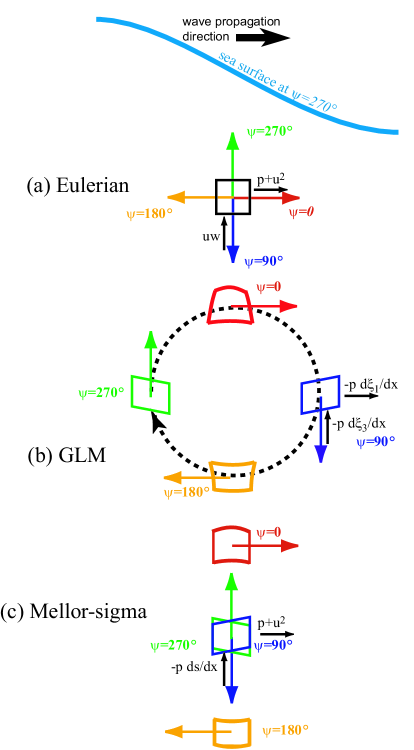
Figure 1: Wave-induced fluxes of horizontal momentum in Eulerian, Generalized Lagrangian, and Mellor-sigma averages of the flow. Viscous or turbulent fluxes are neglected for simplicity. Distorted squares represent an elementary fluid volume and its position at four phases of the wave cycle, and the large arrow indicate the local wave orbital velocity. The horizontal and vertical fluxes of the horizontal momentum are represented by smaller arrows. Their expression are given to lowest order, without Jacobian corrections due to a change of volume (e.g. this results in $u^{2}+p$ becoming Mellor’s $u^{2}+p\partial s/\partial\varsigma$).

Using his coordinate transform, Mellor (2003) obtained a phase-averaged equation for the drift current $U=\widehat{u}+u_{S}$ where $u_{S}$ is the Stokes drift, i.e. the mean velocity of water particles induced by fast wave-induced motions. $U$ is strictly defined as the phase-average particle drift velocity when following the up-and-down wave motion, and $\widehat{u}=U-u_{S}$ is a quasi-Eulerian mean current (Jenkins 1986, 1987). Below the wave crests $\widehat{u}$ is equal, to second order in the wave slope, with the Eulerian mean current $\overline{u}$ (figure 2).

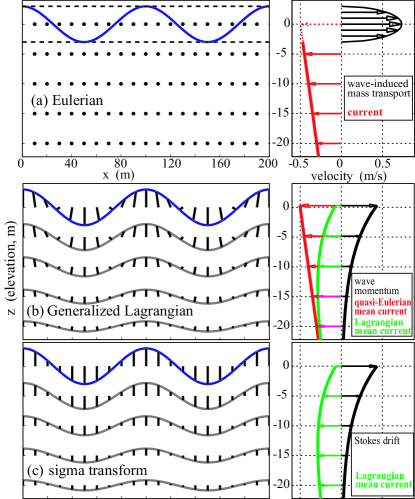
Figure 2: Averaging procedures (left) and examples of resulting velocity profiles (right) in the case of (a) Eulerian averages, (b) the Generalized Lagrangian Mean, (c) sigma transforms (Mellor 2003). The thick black bars connect the fixed points $(x,z)$ where the average field is evaluated, to the displaced points $(x,z)+(\xi_{1},\xi_{3})$ where the instantaneous field is evaluated. For averages in moving coordinates the points $(x,z)+(\xi_{1},\xi_{3})$ at a given vertical level $\xi$ are along the gray lines. The drift velocity is the sum of the (quasi-Eulerian) current and the wave-induced mass transport. In the present illustration an Airy wave of amplitude 3 m and wavelength 100 m in 30 m depth, is superimposed on a hypothetical current of velocity $u(z)=-0.5-0.01z$ m/s for all $z<\zeta(x)$. The quasi-Eulerian current profile is not represented in (c) since it is not directly given in Mellor’s theory, although it can obviously be obtained by taking the difference of the other two profiles.

Mellor’s horizontal mean momentum equation (34a) is reproduced here for completeness, in our conditions with a flow restricted to the vertical $x,z$ plane, a constant water density, no Coriolis force, and no turbulent fluxes and the atmospheric mean pressure set to zero (wind-wave generation due to air pressure fluctuations is absorbed in $F_{x3}$),

$$\frac{\partial DU}{\partial t}+\frac{\partial DU^{2}}{\partial x}+\frac{\partial\Omega U}{\partial\varsigma}+gD\frac{\partial\widehat{\eta}}{\partial x}=F_{xx}+F_{x3}.$$ (5)

On the right-hand the first other term

$$F_{xx}=-\frac{\partial S_{xx}}{\partial x}=-\frac{\partial}{\partial x}\left(\overline{D\widetilde{u}^{2}+\widetilde{p}\frac{\partial\widetilde{s}}{\partial\varsigma}}\right)$$ (6)

represents the convergence of a horizontal flux of horizontal momentum that accelerates the mean drift velocity $U$.

The other term

$$F_{x3}=-\frac{\partial S_{x3}}{\partial\varsigma}=\frac{\partial}{\partial\varsigma}\left(\overline{\widetilde{p}\partial\widetilde{s}/\partial x}\right)$$ (7)

represents a similar convergence of a vertical flux of horizontal momentum.

Defining $g$ as the acceleration due to the apparent gravity, $\widetilde{p}$ and $\widetilde{s}$ are of the order of $ga$ and $a$ respectively. In general $\widetilde{p}$ and $\widetilde{s}$ are almost in phase, thus the flux $S_{x3}$ is of the order of $ga\,\partial a/\partial x$, and the force $F_{x3}$ is of the order of $gDka\,\partial a/\partial x$. Thus, in the case of shoaling waves, $F_{x3}$ is of the order of $gD\varepsilon_{1}^{2}\varepsilon_{2}$.

Mellor estimated the vertical momentum flux $S_{x3}$ from (3) and the corresponding lowest order wave-induced kinematic pressure on $\varsigma$ levels,

$$\widetilde{p}=\widetilde{p}_{0}=ga\left(F_{CC}-F_{SS}\right)\cos(kx-\omega t),$$ (8)

$g$ is the acceleration due to the apparent gravity, and the vertical profile function $F_{CC}$ is defined by

$$F_{CC}=\frac{\cosh\left[kD\right(1+\varsigma\left)\right]}{\cosh\left(kD\right)}=\frac{\cosh\left[k\right(z+h\left)\right]}{\cosh\left(kD\right)}+O(\frac{a}{D}).$$ (9)

For non-dissipating shoaling waves, the right hand side terms of eq. (5) are of order $gD\varepsilon_{1}^{2}\varepsilon_{2}$. The estimation of $F_{x3}$ thus requires the knowledge of $\widetilde{p}/(gD)$ and $k\widetilde{s}$ to order $\varepsilon_{1}\varepsilon_{2}$, for which Airy theory is insufficient. In particular, this estimation demands a formal definition of $\widetilde{s}$, not given by Mellor (2003). Further, eq. (7) is only valid if the wave-induced velocity $\widetilde{\Omega}$ through $\varsigma$ levels is zero, or at least, yields a negligible flux $\overline{\widetilde{\Omega}\widetilde{u}}$ and a negligible mean Jacobian-weighted vertical velocity $\Omega=\overline{\widetilde{\Omega}/(1+\partial s/\partial\varsigma/D)}$. This is not the case over a sloping bottom with Mellor’s (2003) $s$ function.

2.1 Formal definition of the the coordinate change $\widetilde{s}$

For a general surface $\varsigma$ defined implicitly by $z=s(x,\varsigma,t)$, the $\varsigma$ velocity component $\widetilde{\Omega}$ is (e.g. Mellor 2003 eq. 20),

$$\widetilde{\Omega} = \frac{\mathrm{d}(z-s)}{\mathrm{d}t}-\overline{\frac{\mathrm{d}(z-s)}{\mathrm{d}t}}$$ (10)

$$= \widetilde{w}-\widetilde{u}\frac{\partial\overline{s}}{\partial x}-\widehat{u}\frac{\partial\widetilde{s}}{\partial x}-\frac{\partial\widetilde{s}}{\partial t},$$

with $\overline{s}=\overline{\eta}+\varsigma D$.

In the spirit of Mellor’s (2003) derivation, the $\varsigma$ levels should be material surfaces for wave-only motions, so that one may neglect the vertical flux of momentum $\overline{\left(U+\widetilde{u}\right)\widetilde{\Omega}/(1+\partial s/\partial\varsigma/D)}$.

Using the wave-induced vertical and horizontal displacements, $\xi_{3}(x,\varsigma,t)$ and $\xi_{1}(x,\varsigma,t)$, defined by $\partial\xi_{i}/\partial t=\widetilde{u}_{i}(x_{1}+\xi_{1},z+\xi_{3},t)$, we redefine the wave part of $s$,

$$\widetilde{s}^{\prime}\equiv\xi_{3}-\xi_{1}\frac{\partial\overline{s}}{\partial x}.$$ (11)

The first term $\xi_{3}$ corresponds to Mellor’s definition while the second is a $O(\varepsilon_{2})$ relative correction. This definition yields a wave-induced vertical velocity $\widetilde{\Omega}=-\widehat{u}\partial\widetilde{s}^{\prime}/{\partial x}$ through the iso-$\varsigma$ surfaces redefined by $z=s\left(x,\varsigma,t\right)=\overline{\eta}+\varsigma D+\widetilde{s}^{\prime}$. If $\widehat{u}\ll\widetilde{u}$, as in the examples below, then $\widetilde{\Omega}$ is of a higher order compared to that given by Mellor’s (2003) $\widetilde{s}$ (eq. 2).

2.2 Wave-induced vertical displacements and pressure over a sloping bottom

A WKBJ approximation using Airy’s theory is sufficient for estimating $\partial F_{xx}/\partial x$ because the horizontal gradient of any wave-averaged quantity $\phi$ is of order $\varepsilon_{2}k\phi$. On the contrary, the other force $F_{x3}$ is affected by modifications $\widetilde{s}^{\prime}_{1}$ and $\widetilde{p}_{1}$ to the local-flat-bottom solutions $\widetilde{s}^{\prime}$, and $\widetilde{p}$.

For small bottom slopes, $\widetilde{s}^{\prime}_{1}$ and $\widetilde{p}_{1}$ are expected to be of the order of $\varepsilon_{2}\widetilde{s}^{\prime}$ and $\varepsilon_{2}\widetilde{p}$, i.e. of order $a\varepsilon_{2}$ and $ga\varepsilon_{1}\varepsilon_{2}$, respectively. Thus $\partial\widetilde{s}^{\prime}_{1}/\partial x$ is of order $ka\varepsilon_{2}=\varepsilon_{1}\varepsilon_{2}$, and is expected to be in phase with the wave-induced pressure (8), of order $ga$, giving another term of order $gD\varepsilon_{1}^{2}\varepsilon_{2}$ omitted by Mellor in his estimation of $\partial(\overline{\widetilde{p}\partial\widetilde{s}/\partial x})/\partial\varsigma$. The modification of the pressure can be obtained from the modification of the velocity potential, and it may be in phase with $\partial\widetilde{s}_{0}/\partial x$, thus also contributing at the same order to $F_{x3}$.

In order to be convinced of the problem, one may consider the case of steady monochromatic shoaling waves over a slope without bottom friction, viscosity or any kind of surface stress. We also neglect the Coriolis force. In this mathematical experiment, the flow is purely irrotational. We consider that the non-dimensional depth $kH$ is of order 1, and that there is no net mass flux across any vertical section. In that case the mean current and the Stokes drift are of the same order, i.e. of the order $C\varepsilon_{1}^{2}$ with $C$ the phase speed. The mean current exactly compensates the divergence of the wave-induced mass transport, and the mean sea level is lower in the area where the wave height is increased (Longuet-Higgins 1967)

$$\widehat{\eta}(x)=-\frac{kE}{\sinh(2kD)}+\frac{k_{0}E_{0}}{\sinh(2k_{0}D_{0})}$$ (12)

where the $0$ subscript correspond to quantities evaluated at the offshore boundary of the domain.

Since wave forcing is steady, the Eulerian mean current response is steady (e.g. Rivero and Sanchez-Arcilla 1994, McWilliams et al. 2004, Lane et al. 2006), and thus the Lagrangian mean current is also steady. Thus the first term in (5) is zero and the second is of order $DC^{2}\varepsilon_{1}^{4}\varepsilon_{2}/D\simeq gD\varepsilon_{1}^{4}\varepsilon_{2}$. The vertical mean velocity $\Omega$ can be estimated from the steady mass conservation equation,

$$\frac{\partial DU}{\partial x}+\frac{\partial\Omega}{\partial\varsigma}=0$$ (13)

where the first term is of order $DC\varepsilon_{1}^{2}\varepsilon_{2}/D$ and the second is of order $\Omega$. Thus the third term in (5) is of order $C^{2}\varepsilon_{1}^{4}\varepsilon_{2}\simeq gD\varepsilon_{1}^{4}\varepsilon_{2}$. The remaining terms in (5) are of order $\varepsilon_{1}^{2}\varepsilon_{2}$, giving the lowest order momentum balance

$$\stackrel{{\scriptstyle\mathrm{Feta}}}{{-D\frac{\partial}{\partial x}\left(g{\overline{\eta}}\right)}}\stackrel{{\scriptstyle\mathrm{Fxx}}}{{-\frac{\partial S_{xx}}{\partial x}}}+\stackrel{{\scriptstyle\mathrm{Fx3}}}{{\frac{\partial}{\partial\varsigma}\overline{\widetilde{p}\partial\widetilde{s}/\partial x}}}=0.$$ (14)

For reference the corresponding lowest order Eulerian mean balance is (e.g. Rivero and Sanchez-Arcilla 1994, Lane et al. 2006)

$$-\frac{\partial}{\partial x}\left(g{\overline{\eta}}-\overline{\widetilde{w}^{2}}\right)-\frac{\partial\overline{\widetilde{u}^{2}}}{\partial x}-\frac{\partial\overline{\widetilde{u}\widetilde{w}}}{\partial z}=0,.$$ (15)

Only the hydrostatic pressure gradient is present in both the Eulerian and Mellor-sigma balances, because the other terms represent a different balance, including wave momentum in the latter (see figure 2).

Equation (14) is now tested numerically. We take a Roseau-type bottom profile (1976) defined by $x$ and $z$ coordinates given by the real and imaginary part of the complex function

$$Z(x^{\prime})=\frac{h_{1}(x^{\prime}-\mathrm{i}\alpha)+(h_{2}-h_{1})\ln(1+\mathrm{e}^{x^{\prime}-\mathrm{i}\alpha})}{\alpha}.$$ (16)

With $\alpha=15\pi/180$, $h_{1}=6$ m and $h_{2}=4$ m (figure 1), and a radian frequency $\omega=1.2$ rad s^-1 (i.e. a frequency $f=0.2$ Hz), the non-dimensional water depth varies between $0.85<kH<1.1$. The reflection coefficient for the wave amplitude is $1.4\times 10^{-9}$ (Roseau 1976), so that reflected waves may be neglected in the momentum balance. We illustrate the force balance obtained for waves with an offshore amplitude $a_{0}=0.12$ m, which corresponds to a maximum steepness $\varepsilon_{1}=ka=2.6\times 10^{-2}$ equal to the maximum bottom slope $\varepsilon_{2}=\varepsilon_{1}$. The change in wave amplitude is given by the conservation of the wave energy flux (see Ardhuin 2006 for a thorough discussion), and the wave phase $\psi$ is taken as the integral over $x$ of the local wavenumber, so that $\partial\psi/\partial x=k$. The various terms are then estimated using second order finite differences on a regular grid in $\varsigma$ coordinates, with 201 by 401 points covering the domain shown in figure 3.a. The three terms in eq. (14) are shown in figure 3.

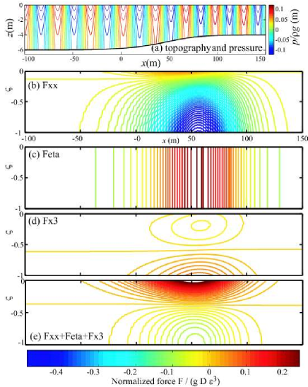
Figure 3: (a) Snapshot of the pressure field for a slowly varying Airy wave over a the bottom topography given by eq. (16). The forces in the balance (14) are shown in panels b, c and d, with their sum in panel e, all estimated from Mellor’s analytical expressions. All forces have been normalized by $gD\varepsilon^{3}$. N.B. in the case shown here $\varepsilon_{1}=\varepsilon_{2}=\varepsilon$.

We have verified that the depth-integrated forces are in balance, within 0.1% of $F_{\mathrm{e}ta}$. However, at most water depths there is a large imbalance, of the order of the individual forces ( i.e. $gD\varepsilon_{1}^{2}\varepsilon_{2}$) ,up to 180% of $F_{\mathrm{e}ta}$. This contradicts the known steady balance obtained from the Eulerian-mean analysis of Rivero and Sanchez-Arcilla (1994).

For the case of shoaling waves without breaking the three-dimensional equations of motion of Mellor (2003) are not consistent to their dominant order, because of an improper approximation of $S_{x3}$. This conclusion holds for any relative magnitude of the wave and bottom slopes $\varepsilon_{1}$ and $\varepsilon_{2}$.

2.3 Wind-forced waves

Clearly, any deviation of the wave-induced fields $s^{\prime}$, $p$, and $u$ from Airy-wave theory may have strong effects on the vertical momentum flux term $S_{x3}$. Another example of such a situation, correctly described by Mellor, is the case of wind-wave generation. We briefly address it here because the full solution can has not been given previously. Mellor focused on the wind-wave generation contribution to the vertical momentum flux term $\widetilde{p}\partial\widetilde{s}/\partial x$ term. This equals the wave-supported wind stress at the sea surface, and, below, it explains the growth of the wave momentum profile with the same profile as that of the Stokes drift (Mellor 2003).

In horizontally uniform conditions, the wave amplitude is a function of time only, and for the sake of simplicity we shall solve the problem in the frame of reference moving at the velocity at which the wave phase is advected by the current. We write the wave-induced non-hydrostatic kinematic Eulerian pressure in the form $\widetilde{p}_{E}=\widetilde{p}_{E0}+\widetilde{p}_{Ew}$, the elevation as $\eta=\zeta_{0}+\zeta_{w}$ and the velocity potential as $\phi=\phi_{0}+\phi_{w}$, in which the 0 subscript refers to the primary waves, and the $w$ subscript refers to the added components in the presence of wind forcing. Taking a primary surface elevation of the form $\zeta_{0}=a\cos\psi$ with the the phase $\psi=kx-\sigma t$, Mellor considered an atmospheric kinematic pressure fluctuation in quadrature with the primary waves

$$\widetilde{p}_{a}=-g\beta\frac{\rho_{w}}{\rho_{a}}a\sin\psi,$$ (17)

with $\beta$ a small non-dimensional wave growth factor, and $\rho_{w}$ and $\rho_{a}$ the densities of water and air respectively. He then assumed that the water-side wave-induced pressure was of the form

$$\widetilde{p}_{\mathrm{Mellor}}=-g\beta a\frac{\cosh\left[k\right(z+h\left)\right]}{\cosh\left(kD\right)}\sin\psi.$$ (18)

Implicitly $\widetilde{s}^{\prime}_{w}$ is zero, and for his purpose $\phi_{w}$ was irrelevant. We shall now also determine $\phi_{w}$. The continuity of dynamic pressures at the surface is

$$\widetilde{p}_{Ew}+g\widetilde{s}^{\prime}_{w}=-g\beta a\sin\psi\quad{\mathrm{at}}\quad z=\zeta.$$ (19)

A solution is obtained by solving Laplace’s equation with proper boundary conditions, to first order in $\beta$. The boundary conditions include the Bernoulli equation,

$$\frac{\partial\phi}{\partial t}=-g\zeta-\frac{\rho_{a}}{\rho_{w}}p_{a},\quad\mbox{at\ }\quad z=\zeta,$$ (20)

in which non-linear terms have been neglected because they are the sum of products of the form $\boldsymbol{\nabla}\phi_{0}\boldsymbol{\cdot}\boldsymbol{\nabla}\zeta_{0}$, unchanged from the case without wind, and terms of the form $\boldsymbol{\nabla}\phi_{w}\boldsymbol{\cdot}\boldsymbol{\nabla}\zeta_{0}$, which are negligible compared to the left-hand side terms for primary waves of small slope. Similarly, the surface kinematic boundary condition is linearized as

$$\frac{\partial\phi}{\partial z}=\frac{\partial\zeta}{\partial t}\quad\mbox{at\ }\quad z=\overline{\zeta}.$$ (21)

The combination of both yields

$$\frac{\partial^{2}\phi}{\partial t^{2}}+g\frac{\partial\phi}{\partial z}=-\frac{\rho_{a}}{\rho_{w}}\frac{\partial\widetilde{p}_{a}}{\partial t}\quad\mbox{at\ }\quad z=\overline{\zeta}.$$ (22)

$\phi_{w}$ is also a solution of Laplace’s equation with the bottom boundary condition $\partial\phi_{w}/\partial z=0$ at $z=-h$. With the fully resonant atmospheric pressure (17) envisaged by Mellor, one has

$$\zeta_{0} = a(t)\cos\psi,$$ (23)

$$\phi_{0} = \frac{ga(t)}{\sigma}F_{CC}\sin\psi,$$ (24)

$${\widetilde{p}}_{E0} = ga(t)F_{CC}\cos\psi,$$ (25)

$$\frac{{\mathrm{d}}a(t)}{{\mathrm{d}}t} = \frac{\beta\sigma a(t)}{2},$$ (26)

$$\phi_{w} = \beta g\frac{a}{2\sigma}F_{CC}\left[A\cos\psi+B\cos\psi^{\prime}\right]$$ (27)

with $\psi^{\prime}=\left(kx+\sigma t\right)$. The elevation and under-water non-hydrostatic pressure corresponding to $\phi_{w}$ are given by (21) and the linearized Bernoulli equation

$$\frac{\partial}{\partial t}\left(\phi_{0}+\phi_{w}\right)=-\widetilde{p}_{E0}-\widetilde{p}_{Ew}$$ (28)

yielding

$$\zeta_{w} = \beta\frac{a}{2}\left[\left(1-A\right)\sin\psi+B\sin\psi^{\prime}\right]$$ (29)

$$\widetilde{p}_{Ew} = g\beta\frac{a}{2}F_{CC}\left[-\left(1+A\right)\sin\psi+B\sin\psi^{\prime}\right].$$

Mellor’s expression for $\widetilde{p}_{w}$ (eq. 18) is obtained by replacing $\zeta_{w}$ and $\widetilde{p}_{Ew}$ in (19), giving $A=1$. One may take $B=1$ to have $\phi_{w}=0$ at $t=0$, or more simply $B=0$, which gives $\zeta_{w}=0$, and $p_{Ew}=F_{CC}\widetilde{p}_{a}\rho_{a}/\rho_{w}$. The choice of $B$ has no dynamical effect. In the present case $\phi_{w}$ should give a contribution to $S_{xx}$ because it is in phase with $\phi_{0}$, but this is a relative correction of order $\beta$, thus negligible. To the contrary, the contribution of $\widetilde{p}_{w}$ to $(\overline{\widetilde{p}\partial\widetilde{s}/\partial x})$ is quite important, because for uniform horizontal conditions this flux is otherwise zero.

3 A solution to the problem ?

Contrary to that particular wind-forcing term, there is no simple asymptotically analytical correction for $\widetilde{p}$ and $\widetilde{s}^{\prime}$ that can account for the bottom slope and wave field gradient. A major problem in this situation is that the wave velocity potential becomes a non-local function of the water depth. The velocity potential and pressure fields may only be investigated analytically for plane beds (e.g. Ehrenmark 2005) or specific bottom profiles. Numerical solutions for the three-dimensional wave motion are generally found as infinite series of modes (e.g. Massel 1993). The velocity potential for any of these modes satisfies Laplace’s equation with a local vertical profile $F_{n}$ proportional to $\cos(k_{n}z+k_{n}h)$ and a dispersion relation $\sigma^{2}=gk_{n}\tan(k_{n}D)$. The local amplitudes of these modes are non-local functions of the water depth, and may be obtained numerically with a coupled-mode model (Massel 1993). This non-local dependance of the wave amplitude on the water depth arises from the elliptic nature of Laplace’s equation, satisfied by the velocity potential in irrotational conditions. The series of modes can be made to converge faster by adding a ‘sloping bottom mode’ that often accounts for a large part of the correction and is a local function of the depth and bottom slope. It is thus of interest to see if that correction only, without the infinite series, may provide a first order analytical correction to Mellor’s momentum flux $S_{x3}$.

Following Athanassoulis and Belibassakis (1999), one may define the velocity potential for that mode as

$$\phi_{1} = -\frac{\mathrm{d}h}{\mathrm{d}x}a\sigma DF(z)\cos\psi,$$ (31)

In order to satisfy the bottom boundary condition $w=\partial\phi_{1}/\partial z=-\frac{\mathrm{d}h}{\mathrm{d}x}\partial\phi_{0}/\partial x$, the function $F$ should verify $D{\mathrm{d}F}(-h)/{\mathrm{d}z}=1/\sinh(kH)$ and the satisfaction of the surface boundary condition may be obtained with $F(0)={\mathrm{d}F}(0)/{\mathrm{d}z}=0$. Athanassoulis and Belibassakis (1999) have used

$$F=F_{\mathrm{AB}}\equiv\frac{1}{\sinh(kD)}\left[\left(\frac{{z}-\overline{\zeta}}{D}\right)^{3}+\left(\frac{{z}-\overline{\zeta}}{D}\right)^{2}\right],$$ (32)

and Chandrasekera and Cheung (2001) have used

$$F=F_{\mathrm{Ch}}\equiv\frac{1}{kD\sinh^{2}(kD)}\left[1-\cosh(k{z}-k\overline{\zeta})\right].$$ (33)

With these choices $\phi_{1}$ does not satisfy exactly Laplace’s equation, and thus requires further corrections in the form of evanescent modes. An infinite number of other choices is available, either satisfying Laplace’s equation or the surface boundary conditions, but never both, so that each of these solutions is only approximate, and the exact solution is given by the infinite series of modes, which can be computed numerically for any bottom topography (e.g. Athanassoulis and Belibassakis 1999, Belibassakis et al. 2001, Magne et al. 2006).

The vertical displacement and Eulerian pressure corrections are given by time integration of the vertical velocity and the linearized Bernoulli equation,

$$\xi_{31} = \frac{\mathrm{d}h}{\mathrm{d}x}aD\frac{\mathrm{d}F}{\mathrm{d}z}\sin\psi$$ (34)

$$\widetilde{p}_{E1} = \frac{\mathrm{d}h}{\mathrm{d}x}aDF(z)\sin\psi$$ (35)

Thus, in absence of wind forcing but taking into account the ‘sloping bottom mode’ to first order in the bottom slope, the wave-induced flux of momentum through iso-$\varsigma$ surfaces is

$$\widetilde{p}\frac{\partial\widetilde{s}^{\prime}}{\partial x}=\left(F_{CC}-F_{SS}\right)\left[\frac{ga}{2}\frac{\partial(aF_{SS})}{\partial x}\right.$$

$$+\left.\frac{gka^{2}}{2}\frac{\mathrm{d}h}{\mathrm{d}x}\left(D\frac{\mathrm{d}F}{\mathrm{d}z}+\varsigma F_{CS}\right)\right]$$

$$+\frac{gka^{2}}{2}\frac{\mathrm{d}h}{\mathrm{d}x}\left[-F_{SC}F+F_{SS}\left(D\frac{\mathrm{d}F}{\mathrm{d}z}+\varsigma F_{CS}\right)\right],$$

with $F_{CS}={\cosh\left[kD\right(1+\varsigma\left)\right]}/{\sinh\left(kD\right)}$. The first line is the term given by Mellor (2003). The second line arises from the correction due to the difference between $\widetilde{s}^{\prime}$ and $\widetilde{s}$, and the third line arises due to corrections $\widetilde{p}_{1}=\widetilde{p}_{E1}-gs^{\prime}_{1}$ to the pressure on $\varsigma$ levels. These additional term are of the same order as the first term, and have no flux at the bottom and surface. Thus the depth-integrated equations including that term also comply with known depth-integrated equations (e.g. Smith 2006).

In the case chosen here $F_{\mathrm{Ch}}$ gives a net momentum balance closer to zero than Mellor’s (2003) original expression (figure 4). However, the remaining error is significant. Thus one cannot use only that mode, and the contribution of the evanescent modes have to be computed, which can only be done numerically.

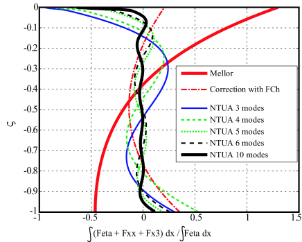
Figure 4: Net forces in the momentum balance (14) for steady shoaling waves over a smooth bottom profile. The net force has been integrated over $x$ and normalized by a similar integration of the the hydrostatic pressure force $F_{eta}$. Several solutions are obtained. One corresponds to Mellor’s orginal expression, one possible analytical correction using $F_{\mathrm{Ch}}$, and numerical estimations using the NTUA model, with various numbers of modes.

A numerical evaluation of the forces was performed using the NTUA model (Athanassoulis and Belibassakis 1999). The NTUA solution was obtained in a domain with 401 points in the horizontal dimension. For the small bottom slope used here, the model contains a numerical reflection $R=0.002$ much larger than the analytical value given by Roseau (1976). However, this only introduces a modulation, in the $x$ direction, of the estimated forces. This modulation is significant but still relatively smaller than the average. The net force estimated from NTUA results is found to converge to the expected force balance described by eq. (14) as the number of evanescent modes is increased (figure 4). In this calculation the values of $F_{xx}$ do not differ significantly from those estimated using Mellor’s analytical expressions, as expected. The only significant difference between the NTUA numerical result with 10 modes, and Mellor’s analytical expression is found in $F_{x3}$, with a much stronger value near the surface in the numerical result, allowing a balance with the strongly sheared $F_{xx}$ (figure 4).

4 Conclusions

Mellor (2003) changed the vertical coordinate from $\varsigma$ to $z$, using an implicit function $s$ in two parts, $z=\overline{s}(x,y,\varsigma,t)+\widetilde{s}(x,y,\varsigma,t)$ with $\overline{s}$ changing only slowly in space and time and $\widetilde{s}$ representing the faster wave-induced change of vertical coordinate. If the $\varsigma$ levels are material surfaces, then the momentum flux $S_{x3}=\widetilde{p}^{\xi}\partial\widetilde{s}/\partial x$ is the surface-following coordinate counterpart of the Eulerian vertical momentum flux term $\overline{\widetilde{u}\widetilde{w}}$ discussed by Rivero and Arcilla (1995), with $\widetilde{p}^{\xi}$ the wave-induced pressure at the displaced position (in the surface-following coordinates). However, $\widetilde{p}^{\xi}\partial\widetilde{s}^{\prime}/\partial x$ and $\overline{\widetilde{u}\widetilde{w}}$ do not represent the same physical quantity since the former contains wave momentum, which is not included in the latter.

Just like the Eulerian momentum flux $\overline{\widetilde{u}\widetilde{w}}$ is modified by the bottom slope, wave amplitude gradients, wind-wave generation, boundary layers, or vertical current shears, these effects also modify $S_{x3}$. But in these situations, the $\varsigma$ levels as defined by Mellor (2003) are not material surfaces, and a missing Eulerian-like flux term $\overline{\widetilde{\Omega}\widetilde{w}}$ would have to be added to correct the momentum equations, with $\widetilde{\Omega}$ the wave-induced velocity across $\varsigma$ levels. Alternatively, we propose to replace $\widetilde{s}$ with $\widetilde{s}^{\prime}$, defined by eq. (11) such that $\varsigma$ levels are closer to material surfaces, i.e. so that $\widetilde{\Omega}$ is of a higher order.

Whether the original $\widetilde{s}$ or our corrected $\widetilde{s}^{\prime}$ is used, the wave-induced momentum flux $S_{x3}$ must be estimated to first order in the bottom slope $\varepsilon_{2}$ for consistency. This requires an $O(\varepsilon_{2})$ estimation of both $\widetilde{p}^{\xi}$ and $\widetilde{s}$ or $\widetilde{s}^{\prime}$. Unfortunately there is no analytical $O(\varepsilon_{2})$ expression for the wave motion. Thus Mellor’s equations, even when corrected, require a computer-intensive solution that is generally not feasible. For example, Magne et al. (2006) only included a total of five modes in their calculation of wave propagation over a submarine canyon. In an example shown here, this small number of modes is insufficient for an accurate estimation of wave-forcing terms.

The trouble with these equations can be avoided by using, instead, equations of motion for the quasi-Eulerian velocity $\widehat{u}=U-u_{S}$ (Jenkins 1986, 1987, 1989). Such equations have been obtained in the limit of vanishing wave amplitude using an analytical continuation (e.g. using a Taylor expansion) of the current profile across the surface (McWilliams et al. 2004). A general and explicit solution can also be obtained from the exact Generalized Lagrangian Mean (GLM) equations of Andrews and McIntyre (1978a) expanded to second order in the surface slope $\varepsilon_{1}$ (Ardhuin et al., manuscript submitted to Ocean Modelling, see [http://arxiv.org/abs/physics/0702067]). In these, the equation for the horizontal quasi-Eulerian momentum involves no flux term like $\overline{\widetilde{p}{\partial\widetilde{s}}/{\partial x}}$ because this corresponds to the flux $\overline{p^{\xi}\partial\xi_{3}/\partial x}[1+O(\varepsilon)]$ of wave momentum $u_{S}$ (Andrews and McIntyre 1978b, eq. 2.7b), not directly relevant to the problem of mean flow evolution (see also Jenkins and Ardhuin 2004). This flux of wave momentum only appears in evolution equations for the total momentum $U$, such as given by Mellor (2003), or the ‘alternative’ form of the GLM equations (Andrews and McIntyre 1978, eq. 8.7a).

For that reason, the equations for the quasi-Eulerian velocity $\widehat{u}$ are simple and consistent in their adiabatic form (without wave dissipation), at least to lowest order in wave slope and current vertical shear, for which analytical expressions exist for the wave forcing terms. Further details on the relationships between all these equations, and further validation against numerical solutions of Laplace’s equation can be found in Ardhuin et al. (submitted manuscript).

Acknowledgments. This work was sparked by a remark of the late and much missed Tony Elfouhaily. The open collaboration of George Mellor and his criticisms of an early draft greatly improved the present note, together with the feedback of anonymous reviewers and many colleagues. Among them Dano Roelvink suggested the evaluation of the torque resulting from Mellor’s equations in the vertical plane, and Jacco Groeneweg made a detailed critique of early drafts. Initiated during the visit of A.D.J. at SHOM, this research was supported by the Aurora Mobility Programme for Research Collaboration between France and Norway, funded by the Research Council of Norway (NFR) and The French Ministry of Foreign Affairs. A. D. J. was supported by NFR Project 155923/700.

References

- Andrews and McIntyre (1978a) Andrews, D. G. and M. E. McIntyre, 1978a: An exact theory of nonlinear waves on a Lagrangian-mean flow. J. Fluid Mech., 89, 609–646.
- Andrews and McIntyre (1978b) — 1978b: On wave action and its relatives. J. Fluid Mech., 89, 647–664, corrigendum: vol. 95, p. 796.
- Ardhuin (2006) Ardhuin, F., 2006: On the momentum balance in shoaling gravity waves: a commentary of shoaling surface gravity waves cause a force and a torque on the bottom by K. E. Kenyon. Journal of Oceanography, 62, 917–922.
- Ardhuin et al. (2005) Ardhuin, F., A. D. Jenkins, D. Hauser, A. Reniers, and B. Chapron, 2005: Waves and operational oceanography: towards a coherent description of the upper ocean for applications. Eos Trans. AGU, 86, 37–39.
- Ardhuin et al. (2004) Ardhuin, F., F.-R. Martin-Lauzer, B. Chapron, P. Craneguy, F. Girard-Ardhuin, and T. Elfouhaily, 2004: Dérive à la surface de l’océan sous l’effet des vagues. Comptes Rendus Géosciences, 336, 1121–1130.
- Athanassoulis and Belibassakis (1999) Athanassoulis, G. A. and K. A. Belibassakis, 1999: A consistent coupled-mode theory for the propagation of small amplitude water waves over variable bathymetry regions. J. Fluid Mech., 389, 275–301.
- Belibassakis et al. (2001) Belibassakis, K. A., G. A. Athanassoulis, and T. P. Gerostathis, 2001: A coupled-mode model for the refraction-diffraction of linear waves over steep three-dimensional bathymetry. Appl. Ocean Res., 23, 319–336.
- Chandrasekera and Cheung (2001) Chandrasekera, C. N. and K. F. Cheung, 2001: Linear refraction-diffraction model for steep bathymetry. J. of Waterway, Port Coast. Ocean Eng., 127, 161–170.
- Ehrenmark (2005) Ehrenmark, U. T., 2005: An alternative dispersion equation for water waves over an inclined bed. J. Fluid Mech., 543, 249 –266.
- Jenkins (1986) Jenkins, A. D., 1986: A theory for steady and variable wind- and wave-induced currents. J. Phys. Oceanogr., 16, 1370–1377.
- Jenkins (1987) — 1987: Wind and wave induced currents in a rotating sea with depth-varying eddy viscosity. J. Phys. Oceanogr., 17, 938–951.
- Jenkins (1989) — 1989: The use of a wave prediction model for driving a near-surface current model. Deut. Hydrogr. Z., 42, 133–149.
- Jenkins and Ardhuin (2004) Jenkins, A. D. and F. Ardhuin, 2004: Interaction of ocean waves and currents: How different approaches may be reconciled. Proc. 14th Int. Offshore & Polar Engng Conf., Toulon, France, May 23–28, 2004, Int. Soc. of Offshore & Polar Engrs, volume 3, 105–111.
- Lane et al. (2007) Lane, E. M., J. M. Restrepo, and J. C. McWilliams, 2007: Wave-current interaction: A comparison of radiation-stress and vortex-force representations. J. Phys. Oceanogr., 37, in press.
- Longuet-Higgins (1967) Longuet-Higgins, M. S., 1967: On the wave-induced difference in mean sea level between the two sides of a submerged breakwater. J. Mar. Res., 25, 148–153.
- Magne et al. (2007) Magne, R., K. Belibassakis, T. H. C. Herbers, F. Ardhuin, W. C. O’Reilly, and V. Rey, 2007: Evolution of surface gravity waves over a submarine canyon. J. Geophys. Res., 112, C01002.
- Massel (1993) Massel, S. R., 1993: Extended refraction-diffraction equation for surface waves. Coastal Eng., 19, 97–126.
- McIntyre (1981) McIntyre, M. E., 1981: On the ’wave momentum’ myth. J. Fluid Mech., 106, 331–347.
- McWilliams et al. (2004) McWilliams, J. C., J. M. Restrepo, and E. M. Lane, 2004: An asymptotic theory for the interaction of waves and currents in coastal waters. J. Fluid Mech., 511, 135–178.
- Mei (1989) Mei, C. C., 1989: Applied dynamics of ocean surface waves. World Scientific, Singapore, second edition, 740 p.
- Mellor (2003) Mellor, G., 2003: The three-dimensional current and surface wave equations. J. Phys. Oceanogr., 33, 1978–1989, corrigendum, vol. 35, p. 2304, 2005.
- Rivero and Arcilla (1995) Rivero, F. J. and A. S. Arcilla, 1995: On the vertical distribution of . Coastal Eng., 25, 135–152.
- Roseau (1976) Roseau, M., 1976: Asymptotic wave theory. Elsevier.
- Smith (2006) Smith, J. A., 2006: Observed variability of ocean wave Stokes drift, and the Eulerian response to passing groups. J. Phys. Oceanogr., 36, 1381–1402.