BILLIARDS, INVARIANT MEASURES, AND EQUILIBRIUM THERMODYNAMICS

V. V. KOZLOV
Department of Mechanics and Mathematics
Moscow State University
Vorob’ievy gory, 119899 Moscow, Russia
E-mail: vako@mech.math.msu.su

The questions of justification of the Gibbs canonical distribution for systems with elastic impacts are discussed. A special attention is paid to the description of probability measures with densities depending on the system energy.

Gibbs Distribution

Let $x=(x_{1},\,\ldots,\,x_{n})$ be generalized coordinates, $y=(y_{1},\,\ldots,\,y_{n})$ be conjugate canonical momenta of a Hamiltonian system with $n$ degrees of freedom and a stationary Hamiltonian $H(x,\,y,\,\lambda)$, where ${\lambda=(\lambda_{1},\,\ldots,\,\lambda_{m})}$ are some parameters. According to Gibbs [1], a distribution with the probability density

$$\rho=ce^{-\beta H},$$ (1)

where $c=const>0,\,\beta=\frac{1}{kT}$ ($T$ is absolute temperature, $k$ is Boltzmann constant) plays a key role in statistical consideration of Hamiltonian systems. The constant $c$ is chosen due to the normalization condition of density $\rho$.

Given an invariant measure with the density (1), we can introduce an mean energy

$$E(\beta,\,\lambda)=\int H\rho\,d^{n}x\,d^{n}y,$$ (2)

and average generalized forces (constraint reactions $\lambda=const$), corresponding to the parameters $\lambda$:

$$\Lambda_{i}=-\int{\frac{\partial{H}}{\partial\lambda_{i}}}\rho\,d^{n}x\,d^{n}y\,,\quad 1\leq i\leq m\,.$$ (3)

Relations $L_{i}=f_{i}(\beta,\,\lambda)$ are considered as equations of state.

As it was shown by Gibbs, 1-form of heat gain

$$\omega=dE+\sum_{1}^{m}\Lambda_{i}\,d\lambda_{i}$$ (4)

satisfies the axioms of thermodynamics: the form $\beta\omega$ is exact ($\beta\omega=dS$, where $S(\beta,\,\lambda)$ is the entropy of a thermodynamical system). In particular, the form $\omega$ is an exact 1-form under fixed values of $\beta$. Thus, according to Gibbs, to any Hamiltonian system (provided that the integrals (2) and (3) exist and depend smoothly on $\lambda$ and $\beta$) there can be associated a thermodynamic system with external parameters $\lambda_{1},\,\ldots,\,\lambda_{m}$, the internal energy (2), and the equations of state (3). The relations (2) and (3) can be simplified by introducing statistical integral

$$Z(\beta,\,\lambda)=\int e^{-\beta H}\,d^{n}x\,d^{n}y\,.$$ (5)

Hence,

$$E=-{\frac{\partial{\ln Z}}{\partial\beta}},\quad\Lambda_{i}=\frac{1}{\beta}{\frac{\partial{\ln Z}}{\partial\lambda_{i}}}$$ (6)

and therefore $\beta\omega=dS$, where

$$S=\ln Z-\beta{\frac{\partial{\ln Z}}{\partial\beta}}\,.$$ (7)

Thermodynamics of Billiards

Billiard is a mass particle performing the inertial motion in domain $D$ of three-dimensional Euclidean space and reflecting elastically from its boundary $\partial D$. We can consider a more general case when there are $n$-identical particles in the domain $D$ not interacting with each other (in particular, not colliding with each other). Such a system is a universally recognized model of rarefied perfect gas.

Let $q_{i}=(x_{i},\,y_{i},\,z_{i})$ be a set of Cartesian coordinates of the i-th particle of unit mass with momentum $p_{i}=(\dot{x}_{i},\,\dot{y}_{i},\,\dot{z}_{i})$. Dynamics of the system in the domain $D$ is defined by a Hamiltonian

$$H=\sum\frac{p_{i}^{2}}{2}\,.$$

Since this function does not contain any information about the geometry of the domain $D$, equations (2) and (3) are not applicable immediately. In this case, one can apply the following procedure: statistical integral (5) is calculated first, and then relations (6) are used. In our case

$$Z=\int_{\mathbb{R}^{3n}}\int_{D^{n}}e^{-\beta H}\,d^{3}p_{1}\ldots d^{3}p_{n}\,d^{3}q_{1}\ldots d^{3}q_{n}=\Bigl{(}\frac{2\pi}{\beta}\Bigr{)}^{\frac{3n}{2}}v^{n}\,,$$

where $v$ is the volume of $D$. Therefore, the only external parameter $\lambda$ is the volume $v$; a conjugate variable $\Lambda$ is the gas pressure $p$ inside $D$. Taking into account (8), from (6) we obtain known equations of a perfect gas

$$E=\frac{3}{2}kT\,,\quad p=\frac{nkT}{v}\,.$$

Billiards, being systems with one-way constraints, are idealization of ordinary mechanical systems with smooth Hamiltonians. When a particle hits the wall, the wall deforms giving rise to great elastic forces which push the particle back into D. These elastic forces are modeled by potential $V_{\nu}(q)$. It equals zero in $D$ and $\frac{\nu f^{2}(q)}{2}$ outside $D$. Here $f$ is a smooth function that defines the boundary equation $\partial D\colon f(q)=0$. The large constant $\nu$ plays a role of elasticity coefficient. It is assumed that the boundary does not contain critical points of the function $f$; in particular, boundary $\partial D$ is a smooth regular surface. As was shown in [2], as $\nu\to\infty$, solutions of a system with the Hamiltonian

$$H=\frac{p^{2}}{2}+V_{\nu}(q)$$

tend to the motions of a system with elastic reflections in $D$.

Application of the Hamiltonian (10) gives corrections to the expression of statistical integral which depend on the area $\sigma$ of the boundary of $D$. Thus, the area $\sigma$ should be as an external parameter of the perfect gas as a thermodynamic system; pressure will be the function of not only volume and temperature, but also of the surface area of a vessel.

The meaning of the correction is that the volume $v$ in (8) is replaced by

$$v+\sqrt{\frac{\pi}{2\nu\beta}}\sigma+O\bigl{(}\nu^{-\frac{3}{2}}\bigr{)}$$

provided that $f$ does not have critical points outside $D$. Taking this fact into account, the equation of internal energy $E$ remains the same and the state equation (9) is replaced by

$$p=\frac{nkT}{v+\sqrt{\varkappa T}\sigma}\,,\quad\varkappa=\frac{\pi k}{\nu}\,.$$

Since $\sigma$ is a new thermodinamical parameter, we should introduce a conjugate variable

$$\eta=\frac{1}{\beta}{\frac{\partial{\ln Z}}{\partial\sigma}}=\frac{nkT\sqrt{\varkappa T}}{v+\sqrt{\varkappa T}\sigma}\,.$$

The relations (12) and (13) constitute a total system of the state equations.

Let us indicate the deduction of the formula (11). To do so, we use an obvious formula

$$\int_{\mathbb{R}^{3}}e^{-\beta V_{\nu}}\,d^{3}q=v+\int_{f\geq 0}e^{-\frac{\beta\nu f^{2}}{2}}d^{3}q\,.$$

According to the saddle-point method, the basic contribution to the asymptotics of the second integral as $\nu\to\infty$ is made by the critical points of the potential $V$. In accordance with the assumption, $df\neq 0$ for $f>0$. Consiquently, a set of critical points coincides with the boundary $\partial D=\{f=0\}$. A non-isolation of the critical points results in a certain difficulty under usual application of the saddle-point method. Let us pass (locally) into a neighdourhood of the boundary to semigeodesical coordinates $u_{1},\,u_{2},\,u_{3}$, where $f\equiv u_{1}$ [3]. In these variables, the Euclidean metric is written in the form

$$du_{1}^{2}+a\,du_{2}^{2}+2b\,du_{2}\,du_{3}+c\,du_{3}^{2}\,,$$

where $a,\,b,\,c$ are smooth functions of $u_{s}$. In these variables the desired integral is replaced asymptotically by the integral

$$\int_{u_{1}\geq 0}g(u_{1})e^{-\frac{\beta\nu u_{1}^{2}}{2}}du_{1}\,,$$

where

$$g=\iint\limits_{\partial D}\sqrt{G}\,du_{2}\,du_{3}\,,\quad G=ac-b^{2}>0\,.$$

Then, with the help of a standard method [4], we obtain the asymptotics of the integral (14):

$$g(0)\sqrt{\frac{\pi}{2\nu\beta}}+O\bigl{(}\nu^{-\frac{3}{2}}\bigr{)}\,.$$

Note now that $g(0)=\sigma$.

Probability Distribution

Now a rigorous deduction of the Gibbs distribution is given only for the case of vanishing interaction of individual subsystems. A classical Darwin-Fauler approach represents an asymptotical (as $n\to\infty$) deduction of Gibbs distribution from the general principles of dynamics in the assumption of the ergodic hypothesis. As it is observed by A. Ya. Hinchin [5], this approach repeats in fact the previous mathematical results, connected with the limiting probability theorems.

In [6] there suggested another deduction of distribution (1). It is based on the fact that the probability density is a single-valued first integral [1]. With the help of Poincaré method, the conditions, under which motion equations of interacting subsystems do not admit integrals of $C^{2}$-class, independent of energy integral, are indicated. These conditions are constructive and, obviously, less strong than the assumption of ergodicity. Moreover, a natural Gibbs postulate about thermodynamical equilibrum of subsystems under vanishing interaction is used in [6].

A statistical analogue of this argument is the deduction of a normal distribution, suggested by Gauss. He does not use the central limiting theorem, but the postulate that a sample mean is an estimate of maximum of probability at the finite number of observations $n\geq 3$ (see [7], [8]).

In connection with the above-said it is usefull to set in order the hierarchy of Hamiltonian dynamical systems with respect to the degree of their arbitrariness. Let us fix the phase space $\mathbb{P}$ of dimention $2n\geq 4$ with analitical structure and introduce into consideration a set $\mathcal{H}$ of all Hamiltonian systems on $\mathbb{P}$ with analytical Hamiltonians. Certainly, it is supposed that the property of Hamiltonians to be analitical on $\mathbb{P}$ is concordant with analytical structure of $\mathbb{P}$ itself.

We introduce a sequence of embedded into each other sets of $\mathcal{H}$:

$$\mathcal{M}\subset\mathcal{E}\subset\mathcal{T}\subset\mathcal{K}^{0}\subset\mathcal{K}^{1}\subset\ldots\subset\mathcal{K}^{\infty}\subset\mathcal{A}\,.$$

Here, $\mathcal{M},\,\mathcal{E}$ and $\mathcal{T}$ are the set of systems, which respectively possess the properties of intermixing, ergodicity and trasitivity on the energy $(2n-1)$-dimentional surfaces. Further, $\mathcal{K}^{s}$ is the set of systems, which do not admit the first integrals of smoothness class of $C^{s}(\mathbb{P})$ not depending on the energy integral. In addition, the case $s=0$ corresponds to the continuous integrals: they are locally unstable on the surfaces of the level of energy integral and take equal values on the trajectories of the Hamiltonian system. The symbol $\mathcal{A}$ denotes Hamiltonian systems, which do not admit an additional analytical integral.

One can deduce an analogous chain of embedded sets for the systems with elastic reflection as well.

First of all we should make sure that the neighbouring sets in the chain (15) do not coincide with each other. The inequalities $\mathcal{M}\neq\mathcal{E}$, $\mathcal{E}\neq\mathcal{T}$, $\mathcal{T}\neq\mathcal{K}^{o}$ can be much easily demonstrated by the examples of area preserving mappings of $T$ of the two-dimentional torus $\mathbb{T}^{2}=\{x,\,y\mod 2\pi\}$. Such mappings can be treated as Poincaré mappings of the energy manifolds cuts of Hamiltonian systems with two degrees of freedom. A classical example of mixing transformation drives an automorphism of a torus, given by a uni-modular matrix

$$\left[\begin{aligned} 2\mbox{ }&1\\ 1\mbox{ }&1\\ \end{aligned}\right].$$

The shifts $x\to x+a$, $y\to y+b$, where numbers $a,\,b$ and $2\pi$ are rationally incommensurable, provide us with known examples of ergodic, but not mixing, transformations. Thus, $\mathcal{M}\neq\mathcal{E}$. It is considerably more difficult to give examples of transitive, but not ergodic, transformations with an invariant measure. For the first instances of such transformations we cite the work by L. G. Shnirelman (1930) and A. Bezikovich (1937). They considered continuous automorphisms of a circle. Smooth modifications of such transformations are indicated in [9].

To proof the inequality $\mathcal{T}\neq\mathcal{K}^{o}$ we use an example of transitive area preserving transformation $T$ of the square $K^{2}$ which leaves the points on its boundary immovable. Such an example is built by Oxtoby [10] with the help of theory of categories of sets. Let us take four such squares and form one square of quadruplicated area out of the four (see Figure 1). Identifying opposite sides, we will obtain two-dimentional torus, where the mapping $T\colon K^{2}\to K^{2}$ is naturally prolonged to the contituous area-preserving mapping $T\colon\mathbb{T}^{2}\to\mathbb{T}^{2}$. We need hardly mention that this transformation will no longer be transitive. Still it does not admit non-constant continuous integrals. It would be interesting to provide an analytical example of the transformation from the set of $\mathcal{K}^{o}\setminus\mathcal{T}$.

Inequalities $\mathcal{K}^{k}\neq\mathcal{K}^{k+1}(k=0,\,1,\,\ldots,\,\infty)$ and $\mathcal{K}^{\infty}\neq\mathcal{A}$ are derived from the results of [11] (see also [12]), where the examples of analytical Hamiltonian systems, not possessing additional integrals of $C^{k}(C^{\infty})$–class, but at same time not admitting integrals of $C^{k+1}\bigl{(}C^{\omega}\bigr{)}$–class, are indicated.

Let us consider one of the links of the chain of inclusions of (15), say, $\mathcal{T}\subset\mathcal{K}^{o}$. The question is, which of the two sets is more massive: $\mathcal{T}$ or $\mathcal{K}^{o}\setminus\mathcal{T}$. Apparently, the second. However, the answer to this question (as well as its formulation) depends on the introduced topology in the space $\mathcal{K}^{o}$. Analogous assumptions are probably valid for any pair of the neighbouring sets in (15).

Classes of systems from (15) may be laid out into a wider class of systems, which do not admit additional single-valued complex-analytic first integrals. An obstacle to the existence of single-valued holomorphic integrals is the branching of the solutions of Hamiltonian systems in the plane of complex time. The discussion of this range of questions one can find in the work [13].

If we remain within the real examination, then the class $\mathcal{A}$ admits a natural extension for the dynamics of natural machanical systems. They are decribed by the Hamiltonians of the form $H=T+V$, where $T$ is a kinetic energy, a positively defined quadratic form with respect to the momenta, and $V$ is a potential energy, a function on the configuration space. All known integrals of such systems are polynomials in momenta with single-valued, coefficients on configuration space, (or functions of such polynomials). In analytical case, these coefficients are also represented by analytical functions. We can show that the existence of an additional polynomial integral of the system with the Hamiltonian $H=T+V$ is equivalent to the existence of an integral of the system with the Hamiltonian $H=T+\varepsilon V$ ($\varepsilon$ is a small parameter) as the series in terms of powers of $\varepsilon$.

This problem is more simple and since Poincaré times there have been proposed efficient methods for its solution [13]. The existence conditions of additional polynomial integral of a plane billiard are obtained with the help of complex variable function [14].

The issue of whether a certain Hamiltonian system belongs to the class $\mathcal{A}$ is more complex. But essential advances have been made in this field as well, especially for the case with small number of degrees of freedom [13]. Difficulties become much more severe as we move towards the beginning of the chain (15). Thus, according to Kac [15], an efficient verification of the ergodic property of a dynamical system is a nearly hopeless problem. Moreover, in many important cases, from the application viewpoint, ergodic hypothesis is refuted by the results of KAM theory. For instance, as it was established by Lazutkin [16], a billiard inside a plane convex curve (of $C^{2}$–class of smoothness) is not ergodic. It does not even possess the transitive property. Lack of ergodicity in spatial case was proved in [17] under some additional conditions. These examples are directly related with the deduction of Gibbs distribution for the perfect gas.

For small perturbation of an integrable Hamiltonian system with two degrees of freedom, Kolmogorov tori cut a three-dimentional energy surfaces. Therefore, a perturbed system can no longer be transitive. On the other hand, as it was noted by Arnold, such systems admit a nonconstant continuous integral that takes constant values in slits between Kolmogorov tori. It’s not quite clear yet whether such systems have locally nonconstant continuous first integrals which are not identically constant in any neighbourhood of every point of the energy surface. A simpler problem is whether perturbed systems of general kind with two degrees of freedom admit nonconstant integrals of $C^{1}$–smoothness class.

For systems with $n\geq 3$ degrees of freedom, the slits between Kolmogorov tori form a connected set everywhere densely filling a five–dimensional energy manifolds. Therefore, a principal possibility of the appearance of transitive property arises. This is one of the exact statements of the known hypothesis of diffusion in perturbated multidimensional Hamiltonian systems. For the purpose of statistical mechanics this diffusion hypothesis can be formulated in a less restricted fashion: is it true that under great $n$ a perturbed Hamiltonian system of general form does not admit nonconstant continuous (or even smooth, of $C^{1}$–class) first integrals on ($2n-1$)-dimensional energy surfaces? In fact, it is sufficient that this property appeared under a small fixed value of perturbing parameter $\varepsilon$ and a great value of $n$ of weakly interacting subsystems.

Generalized entropy

Our observations described in previous Section result in a natural assumption that the density of probability distribution $\rho$ is a function of $H$. The question is: what makes Gibbs distribution different from all other distributions of this kind?

Let $z\to f(z)$ be a nonnegative real function of one variable, $f^{\prime}$ be its derivative. Following Gibbs, we will consider probability density

$$\rho=\frac{f(\beta H)}{\int f(\beta H)\,dx\,dy}$$

assuming that the integral converges over the whole phase space. Here again $\beta^{-1}=kT$. When $f=ce^{-z},\,c=const\neq 0$, we shall obtain Gibbs distribution. We could consider a more general case, when the function $f$ depends also on external parameters $\lambda$ (as well as the Hamiltonian $H$). But we shall not follow this case.

Let us calculate an average energy $E$ and generalized forces $\Lambda$ using (2) and (3), with density $\rho$ determined by (16). Then we can compose 1-form of heat gain in accordance with (4). Using direct calculations we can prove

Theorem. The form $\omega$ satisfies axioms of thermodynamics if

$$\int\frac{\partial{H}}{{\partial\lambda_{i}}}f\,dx\,dy\int\frac{\partial{H}}{{\partial\lambda_{j}}}f^{\prime}\,dx\,dy=\int\frac{\partial{H}}{{\partial\lambda_{j}}}f\,dx\,dy\int\frac{\partial{H}}{{\partial\lambda_{i}}}f^{\prime}\,dx\,dy\,.$$

for all $1\leq i,\,j\leq m$ and

$$\int Hf\,dx\,dy\,\int\frac{\partial{H}}{{\partial\lambda_{i}}}f^{\prime}\,dx\,dy=\int\frac{\partial{H}}{{\partial\lambda_{i}}}f\,dx\,dy\,\int Hf^{\prime}\,dx\,dy$$

for all $1\leq i\leq m$.

It is obvious that for the function $f(z)=ce^{-z}$ these conditions are met. Equalities (17) and (18) can be rewritten as follows

$$\Lambda_{i}\frac{\partial{F}}{{\partial\lambda_{j}}}=\Lambda_{j}\frac{\partial{F}}{{\partial\lambda_{i}}}\,,\quad(1\leq i,\,j\leq m)\,,$$

$$\frac{E}{\beta}\frac{\partial{F}}{\partial\lambda_{i}}=-\Lambda_{i}\frac{\partial{F}}{{\partial\beta}}\,,\quad(1\leq i\leq m)\,,$$

where

$$F=\int f(\beta H)d^{n}x\,d^{n}y\,.$$

By analogy with Gibbs case, the function $F$ can be called a generalized statistical integral.

From (19) and (20) follows the existence of function $x(\beta,\,\lambda_{1},\,\ldots,\,\lambda_{m})$, such that

$$\Lambda_{i}=-\frac{\varkappa}{\beta}\frac{\partial{F}}{\partial\lambda_{i}}\,,\quad E=\varkappa\frac{\partial F}{\partial\beta}\,.$$

Therefore, the form of heat gain takes the form

$$\omega=d\Bigl{(}\varkappa\frac{\partial F}{\partial\beta}\Bigr{)}-\sum\frac{\varkappa}{\beta}\frac{\partial{F}}{\partial\lambda_{i}}\,d\lambda_{i}\,.$$

Axioms of thermodynamics impose constraints on the form of function $x$. From (19) we obtain a series of inequalities

$$\frac{\partial{\varkappa}}{\partial\lambda_{i}}\frac{\partial{F}}{\partial\lambda_{j}}-\frac{\partial{\varkappa}}{\partial\lambda_{j}}\frac{\partial{F}}{\partial\lambda_{i}}=0\,,\quad(1\leq i,\,j\leq m)\,,$$

and the equation (20) yields relations

$$\frac{\partial{\varkappa}}{\partial\beta}\frac{\partial{F}}{\partial\lambda_{j}}-\frac{\partial{\varkappa}}{\partial\lambda_{i}}\frac{\partial{F}}{\partial\beta}=0\,,\quad(1\leq i\leq m)\,.$$

Equalities (22) and (23) denote that functions $\varkappa$ and $F$ are dependent. Therefore, we can write that $\varkappa=\varkappa(F)$, at least locally.

Let $\Phi$ be antiderivative of $\varkappa(\cdot)$. Then equalities (21) take a simpler form

$$\Lambda_{i}=-\frac{1}{\beta}\frac{\partial{\Phi}}{\partial\lambda_{i}}\,,\quad E=\frac{\partial{\Phi}}{\partial\beta}\,.$$

Hence

$$\beta\omega =\beta\,d\Bigl{(}\frac{\partial{\Phi}}{\partial\beta}\Bigr{)}-\sum\frac{\partial{\Phi}}{\partial\lambda_{i}}\,d\lambda_{i}=$$

$$=d\Bigl{(}\beta\frac{\partial{\Phi}}{\partial\beta}\Bigr{)}-\frac{\partial{\Phi}}{\partial\beta}\,d\beta-\sum\frac{\partial{\Phi}}{\partial\lambda_{i}}\,d\lambda_{i}=$$

$$=d\Bigl{(}\beta\frac{\partial{\Phi}}{\partial\beta}-\Phi\Bigr{)}\,.$$

The function

$$S=\beta\frac{\partial{\Phi}}{\partial\beta}-\Phi$$

is called an entropy in thermodynamics.

The form of this function suggests that Legendre transform over $\beta$ should be applied. Assuming that

$$\frac{{\partial}^{2}\Phi}{\partial\beta^{2}}\neq 0\,,$$

from the second relation of (24) we will obtain $\beta$ as a function of $E$ and $\lambda$. We will assume $E,\,\lambda_{1},\,\ldots,\,\lambda_{m}$ independent variables. Then $S=S(E,\lambda)$ and from (25) we will obtain potential form of basic thermodynamic relations (24):

$$\beta=\frac{\partial S}{\partial E},\quad\beta\Lambda_{i}=\frac{\partial{S}}{\partial\lambda_{i}}\quad(1\leq i\leq m).$$

The Perfect Gas

Let us apply relations from previous Section to the perfect gas inside domain $D$ of the three-dimentional Euclidean space; let $v$ be the volume of $D$. Remembering that the perfect gas is a totality of $n$ equal and not interacting particles performing the inertial motion inside $D$ and reflecting elastically from its boundary $\partial D$. When taking into account arbitrarily small interaction of particles, we will obtain a system without additional integrals and therefore we can consider that the density of probability distribution is a function of total energy. Let particle interaction tends to zero; then we will obtain simple equations for average energy and state equations; these equations define thermodynamics of a simplified system, i. e. the perfect gas. Let particle mass be equal to unit. Hence, the Hamiltonian for the perfect gas will be determined by the following equation

$$H=\sum\frac{p_{i}^{2}}{2}\,,$$

where $p_{i}=(\dot{x}_{i},\dot{y}_{i},\dot{z}_{i})$ is momentum of the $i$-th particle; let $q_{i}=(x_{i},\,y_{i},\,z_{i})$ be its Cartesian coordinates.

The formula for internal energy has the form

$$E=\frac{\int_{\mathbb{R}^{3n}}\int_{D^{n}}\frac{1}{2}\sum p_{i}^{2}f\Bigl{(}\frac{\beta}{2}\sum p_{i}^{2}\Bigr{)}\,d^{3n}p\,d^{3n}q}{\int_{\mathbb{R}^{3n}}\int_{D^{n}}f\Bigl{(}\frac{\beta}{2}\sum p_{i}^{2}\Bigr{)}\,d^{3n}p\,d^{3n}q}\,.$$

It is independent of volume $v$:

$$E(\beta)=\frac{a}{b\beta}\,,$$

where

$$a =\int_{\mathbb{R}^{3n}}\frac{1}{2}\sum u_{i}^{2}f\Bigl{(}\frac{1}{2}\sum u_{i}^{2}\Bigr{)}\,d^{3n}u\,,$$

$$b =\int_{\mathbb{R}^{3n}}f\Bigl{(}\frac{1}{2}\sum u_{i}^{2}\Bigr{)}\,d^{3n}u\,.$$

Variables $p$ and $u$ are connected by simple relations: $u_{i}=\sqrt{\beta}p_{i}$.

Assuming for simplicity $3n=m+2$, we will pass from $u_{1},\,\ldots,\,u_{m+2}$ to spherical coordinates $r,\,\theta_{1},\,\dots,\,\theta_{m},\,\varphi$ using the following equations

$$u_{1} =r\cos\theta_{1}\,,$$

$$u_{2} =r\sin\theta_{1}\cos\theta_{2}\,,$$

$$u_{3} =r\sin\theta_{1}\sin\theta_{2}\cos\theta_{3}\,,$$

$$\ldots \ldots\ldots\ldots\ldots\ldots\ldots\ldots\ldots$$

$$u_{m} =r\sin\theta_{1}\sin\theta_{2}\ldots\sin\theta_{m-1}\cos\theta_{m}\,,$$

$$u_{m+1} =r\sin\theta_{1}\sin\theta_{2}\ldots\sin\theta_{m}\cos\varphi\,,$$

$$u_{m+2} =r\sin\theta_{1}\sin\theta_{2}\ldots\sin\theta_{m}\sin\varphi\,.$$

Here $r\geq 0,\,0\leq\theta_{j}\leq\pi\,(1\leq j\leq m)$ and $\varphi\mod 2\pi$ is an angular coordinate.

In the new coordinates

$$b={} \int_{0}^{\infty}r^{m+1}f\Bigl{(}\frac{r^{2}}{2}\Bigr{)}\,dr\int_{0}^{\pi}\dots\int_{0}^{\pi}\int_{0}^{2\pi}(\sin\theta_{1})^{m}(\sin\theta_{2})^{m-1}\ldots(\sin\theta_{m})\,d\theta_{1}\dots d\theta_{m}\,d\varphi=$$

$$={} \frac{2\pi^{1+\frac{m}{2}}}{\Gamma\Bigl{(}1+\frac{m}{2}\Bigr{)}}\int_{0}^{\infty}r^{m+1}f\Bigl{(}\frac{r^{2}}{2}\Bigr{)}\,dr\,,$$

where $\Gamma$ is Euler’s gamma-function. By analogy,

$$a=\frac{2\pi^{1+\frac{m}{2}}}{\Gamma\Bigl{(}1+\frac{m}{2}\Bigr{)}}\int_{0}^{\infty}\frac{r^{m+3}}{2}f\Bigl{(}\frac{r^{2}}{2}\Bigr{)}\,dr\,.$$

Now we calculate generalized statistical integral:

$$F=\int_{\mathbb{R}^{3n}}\int_{D^{n}}f\Bigl{(}\frac{\beta}{2}\sum p_{i}^{2}\Bigr{)}\,d^{3n}p\,d^{3n}q=\frac{bv^{n}}{(\sqrt{\beta})^{3n}}\,.$$

According to (21)

$$E=\varkappa\frac{\partial{F}}{\partial\beta}\,.$$

Therefore, taking into account (26) and (29),

$$\varkappa=-\frac{2a(\sqrt{\beta})^{3n}}{3nb^{2}v^{n}}\,.$$

Applying the first equation (21), we obtain state equations

$$\Lambda=-\frac{\varkappa}{\beta}\frac{\partial{F}}{\partial v}=\frac{2a}{3bv\beta}\,.$$

Denoting pressure $\Lambda$ by $p$ in accordance with established thermodynamical notation, we arrive at a more usual form of state equation:

$$pv=\frac{2}{3}\frac{a}{b}kT\,.$$

Now let $f(z)=e^{-z}$. Thus,

$$b=\frac{1}{m+2}\int_{0}^{\infty}e^{-\frac{r^{2}}{2}}\,dr^{m+2}=\frac{2a}{m+2}\,.$$

Hence, $\frac{a}{b}=\frac{(m+2)}{2}=\frac{3n}{2}$ and state equation (30) trnasforms into the classical Clapeyron equation:

$$pv=nkT\,.$$

Now assuming that state equations (30) and (31) are identical under any $n$, we can ask the following question. Is it true that frequency function will be of Gibbs form, i. e. $f(z)=\exp(-z)$? The answer appears to be negative. Actually, (30) and (31) are identical if

$$\frac{a}{b}=\frac{3n}{2}=\frac{m+2}{2}\,,\quad m=3n-2=1,\,4,\,7,\,\ldots\,.$$

With account of (27) and (28) these equations take the following form

$$\int_{0}^{\infty}r^{m+3}f\Bigl{(}\frac{r^{2}}{2}\Bigr{)}dr=(m+2)\int_{0}^{\infty}r^{m+1}f\Bigl{(}\frac{r^{2}}{2}\Bigr{)}dr\,.$$

Let $f$ be decreasing at infinity faster than any exponential function. Then by part-wise integrating we can represent (32) as follows

$$\int_{0}^{\infty}\Bigl{[}f^{\prime}\Bigl{(}\frac{r^{2}}{2}\Bigr{)}+f\Bigl{(}\frac{r^{2}}{2}\Bigr{)}\Bigr{]}r^{m+3}\,dr=0$$

for all $m+3=3n+1=4,\,7,\,10,\,\ldots$. If this equality was true for all non-negative $m+3$, then according to classical momenta theory [18], the expression in the square brackets of (33) would be equal to zero. Hence $f^{\prime}+f=0$ and, therefore, $f=ce^{-z},\,c=const$. However, (33) is not valid for the “majority” of integer values of $m+3$. Hence, it follows that there is an infinite-dimensional space of frequency functions dependent on total energy only, which result in classical thermodynamical relations for the perfect gas.

The work has been partially supported by RFBR (grant No. 99-01-0196) and INTAS (grant No. 96-0799) foundations.

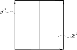
Figure 1:

References

- [1] G. V. Gibbs. Thermodynamics. Statistical Mechanics. Moscow, Nauka, 1982, P. 384.
- [2] V. V. Kozlov. A Constructive Method of Justification of the Theory of Systems with Unilateral Constraints. Prikl. Mekh. i Mat., 1988, V. 52, Iss. 6, P. 883-894.
- [3] P. K. Rashevsky. Riemannian Geometry and Tensor Analysis. Moscow, Nauka, 1967, P. 664.
- [4] N. G. Brain. Asymptotic Methods in Analysis. Moscow, IL, 1961, P. 247.
- [5] A. Ya Hinchin. Mathematical Grounds for Statistical Mechanics. Moscow–Leningrad, Gostekhizdat, 1943, P. 128.
- [6] V. V. Kozlov. Canonical Gibbs Distribution and Thermodynamics of Mechanical Systems with a Finite Number of Degree of Freedom. Regular and Chaotic Dynamics, 1999, V. 4, No. ,2, P. 44–54.
- [7] E. T. Whittaker, G. Robinson. The Calculus of Observations. Blackil and Son, 1928.
- [8] A. M. Kachan, Yu. V. Linnik, S. R. Rao. Characterizational Problems of Mathematical Statistics. Moscow, Nauka, 1972, P. 656.
- [9] E. A. Sidorov. Smooth Topological Transitive Systems. Mathematical Notes, 1968, V. 4, No. 6, P. 751–759.
- [10] J. C. Oxtoby. Note of Transitive Transformations. Proc. Mat. Acad. Sci. U.S., 1937, V. 23, P. 443–446.
- [11] V. V. Kozlov. Phenomena of Nonintegrability in Hamiltonian Systems. Proc. Int. Congr. Math. Berkeley. California. USA, 1987, P. 1161–1170.
- [12] N. G. Moshchevitin. On Existence and Smoothness of an Integral of a Hamiltonian System with a Defined Form. Mathematical Notes, 1991, V. 49, No. 5, P. 80–85.
- [13] V. V. Kozlov. Symmetries, Topology and Resonances in Hamiltonian Mechanics. Springer–Verlag, 1996, P. 378.
- [14] S. V. Bolotin. Birkhoff Integrable Billiards. Vestnik MGU, Ser. Mat., Mekh., 1990, No. 2, P. 33–36.
- [15] M. Kac. Probability and Related Topics in Physical Sciences. Intersience Publishers, 1957.
- [16] V. F. Lazutkin. A Convex Billiard and Eigenfunctions of the Laplace Operator. Leningrad, LGU Publishers, 1981, P. 196.
- [17] N. V. Svanidze. Existence of Invariant Tori for a Three-Dimentional Billiard Located in a Neighbourhood of a “Closed Geodesic on the Domain Boundary”. UMN, 1978, V. 33, Iss. 4, P. 225–226
- [18] N. I. Ahieser. Classical Problem of Moments. Moscow, Nauka, 1961, P. 310.