The effects of spatial constraints on the evolution of weighted complex networks

Abstract

Motivated by the empirical analysis of the air transportation system, we define a network model that includes geographical attributes along with topological and weight (traffic) properties. The introduction of geographical attributes is made by constraining the network in real space. Interestingly, the inclusion of geometrical features induces non-trivial correlations between the weights, the connectivity pattern and the actual spatial distances of vertices. The model also recovers the emergence of anomalous fluctuations in the betweenness-degree correlation function as first observed by Guimerà and Amaral [Eur. Phys. J. B 38, 381 (2004)]. The presented results suggest that the interplay between weight dynamics and spatial constraints is a key ingredient in order to understand the formation of real-world weighted networks.

I Introduction

The empirical evidence coming from studies on systems belonging to areas as diverse as social sciences, biology and computer science have shown that the usual paradigm of random graphs is often not well suited to describe real world networks barabasi:2002 ; dorogovtsev:2002 ; mdbook ; psvbook . In particular, in a wide range of networks the occurrence of vertices with a very large degree (number of links to other vertices) is very likely. The presence of these “hubs” often goes along with very large degree fluctuations. The large topological heterogeneity associated to these features is statistically expressed by the presence of heavy-tailed degree distributions with diverging variance that have a very strong impact on the networks’ physical properties such as resilience and vulnerability, or the propagation of pathogen agents havlin00 ; newman00 ; barabasi00 ; pv01a .

The purely topological definition of networks, however, misses important attributes which are frequently encountered in real-world networks. In the first instance, networks are far from boolean structure and are better represented as weighted graphs with the intensity of links that may vary over many orders of magnitude. Indeed, in many graphs ranging from food-webs to metabolic networks, large variations of the link intensities are empirically observed  granovetter:1973 ; garla:2003 ; li:2003a ; li:2003b ; krause:2003 ; barrat:2004a ; almaas:2004 . Notably, the statistical properties of weights indicate non-trivial correlations and association with topological quantities barrat:2004a . Finally, the correlation between weights on different links is at the origin of the existence of pathways which are particularly important in metabolic networks for example almaas:2004 . Another important element of many real networks is their embedding in the real space. For instance, most people have their friends and relatives in their neighborhood, transportation networks depend on distance, and many communication networks devices have short radio range helmy02 ; nemeth02 ; gorman03 ; Gastner:2004a ; Gastner:2004b . A particularly important example of such a “spatial” network is the Internet which is a set or routers linked by physical cables with different lengths and latency times lakhina02 ; psvbook . An analogous situation is faced in the air transportation network with routes covering very different distances. The length of the link is a very important quantity usually associated with an intrinsic cost in the establishment of the connection. If the cost of a long-range link is high, most of the connections starting from a given node will go to the closest neighbors in the embedding space. Long-range links, on the other hand, correspond usually to connections towards already well-connected nodes (hubs). This seems natural in the case of the air transportation network for instance: short connections go to small airports while long distance flights are directed preferentially towards large airports (i.e. well connected nodes). It is therefore natural to find that spatial constraints can have important consequences on the topology of the resulting network barthelemy:2003a ; amaral:2004 .

Recently, the raising interest on the dynamics and function of complex networks has fostered studies going beyond the simple topological structure. In particular, models of complex networks in which the diversity of weights is taken into account have been formulated having in mind growing networks where the dynamics is driven by the intensity of the weights along with a reinforcement mechanism  barrat:2004b ; barrat:2004c ; barrat:2004d ; pandya:2004 . Other models have focused on more geometrical mechanisms or somehow different dynamical rules dorogovtsev:2004 ; krapivsky:2004 ; bianconi:2004 ; wang:2005 . These models, however, are not able to reproduce all of the features observed in real world networks. For instance, the anomalous centrality fluctuations observed in Ref. amaral:2004 do not find a rationalization in models based only on topology and weight properties. On the other hand, some of these interesting and non-trivial features can result from the introduction of spatial attributes in the models’ construction amaral:2004 . In this article, we discuss the interplay of the three aforementioned ingredients (heterogeneous topology, weights and spatial constraints) in a model of growing network combining these ingredients at once. The proposed model is obtained as the embedding of the weighted growing network introduced in barrat:2004b in a two-dimensional geometrical space. Spatial constraints are translated into a preference for short links, and combined with the coupling between the evolution of the network and the dynamical rearrangement of the weights. This mechanism naturally leads to the appearance of many features observed in real-world networks, in particular the non-linear correlations between weights and topology, and the large fluctuations of the betweenness centrality.

The paper is organized as follows. In section II, we briefly review some important empirical results of the North-American airline network, highlighting the most salient effects on space on different quantities. Sections III and IV are devoted to the presentation and to the study of the spatial weighted model, stressing the effect of the spatial embedding and constraints on the properties of the resulting network. In section V, we present a summary of the results and conclusions about large network modeling.

II A case study: Space, topology and traffic in the North American airline network

The airline transportation infrastructure is a paramount example of large scale network which can be represented as a complex weighted graph: the airports are the vertices of the graph and the links represent the presence of direct flight connections among them. The weight on each link is the number of maximum passengers on the corresponding connection. The characteristics of the world-wide air-transportation network using the International Air Transportation Association (IATA) database IATA have been presented in barrat:2004a . The network is made of $N=3880$ vertices and $E=18810$ edges and shows both small-world and scale-free properties as also confirmed in different datasets and analyses li:2003a ; li:2003b ; guimera:2003 ; amaral:2004 . In particular, the average shortest path length, measured as the average number of edges separating any two nodes in the network shows the value $\langle\ell\rangle=4.37$, very small compared to the network size $N$. The degree distribution, takes the form $P(k)=k^{-\gamma}f(k/k_{x})$, where $\gamma\simeq 2.0$ and $f(k/k_{x})$ is an exponential cut-off function. The degree distribution is therefore heavy-tailed with a cut-off that finds its origin in the physical constraints on the maximum number of connections that a single airport can handle guimera:2003 ; amaral:2004 ; amaral:2000 . The airport connection graph is therefore a clear example of small-world network showing a heavy-tailed degree distribution and heterogeneous topological properties.

The world-wide airline network necessarily mixes different effects. In particular there are clearly two different scales, global (intercontinental) and domestic. The intercontinental scale defines two different groups of travel distances and for the statistical consistency we eliminate this specific geographical constraint by focusing on a single continental case. Namely, in the following we will consider the North-American network constituted of $N=935$ vertices with an average degree $\langle k\rangle\approx 8.4$ and an average shortest path $\ell\approx 4$. The statistical topological properties of the North American network are consistent with the world-wide one as we will see in the forthcoming analysis.

II.1 Topology and weights

The North American network presents a degree distribution statistically consistent with the world-wide airline network. Indeed, we also observe (Fig. 1) in this case a power-law behavior on almost two orders of magnitude followed by a cut-off indicating the maximum number of connections possible due to limited airport capacity and to the size of the network considered.

The existence of a broad degree distribution signals a strong heterogeneity of the network at the topological level which exists also at the weight level.

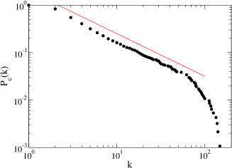
Figure 1: Cumulative degree distribution $P_{c}(k)$ for the North-American network. The straight line indicates a power-law decay with exponent $\gamma-1=0.9$.

A first indication on the weight heterogeneity is given by the study of the weight strength of a node $i$ as defined by yook:2001 ; barrat:2004a

$$s_{i}^{w}=\sum_{j\in{\cal V}(i)}w_{ij}\ .$$ (1)

where the sum runs over the set ${\cal V}(i)$ of neighbors of $i$. The strength generalizes the degree to weighted networks and in the case of the air transportation network quantifies the traffic of passengers handled by any given airport. This quantity obviously depends on the degree $k$ and increases (linearly) with $k$ in the case of random uncorrelated weights of average $\langle w\rangle$. A relation between the average strength $s^{w}(k)$ of nodes of degree $k$ of the form

$$s^{w}=Ak^{\beta_{w}}\ ,$$ (2)

with an exponent $\beta_{w}>1$, or $\beta_{w}=1$ but $A\neq\langle w\rangle$ is then the signature of non-trivial statistical correlations between weights and topology. This is indeed what we observe in the North-American air transportation network with $\beta_{w}\simeq 1.7$ (Fig. 2).

II.2 Spatial analysis

The spatial attributes of the North American airport network are embodied in the physical spatial distance, measured in kilometers or miles, characterizing each connection. Fig. 3 displays the histogram of the distances of the direct flights. These distances correspond to Euclidean measures of the links and clearly show a fast decaying behavior reasonably fitted by an exponential. The exponential fit gives a value for a typical scale of the order $1000$ kms. The origin of the finite scale can be traced back to the existence of physical and economical restrictions on airline planning in a continental setting.

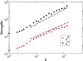
Figure 2: Weight and distance strengths versus degree for the North-American network. The dashed lines correspond to the power-laws $\beta_{d}\simeq 1.4$ and $\beta_{w}\simeq 1.7$.

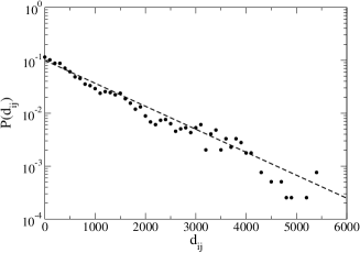
Figure 3: Distribution of distances (in kms) between airports linked by a direct connection for the North-American network. The straight line indicates an exponential decay with scale of order $1000$ km.

Since space is an important parameter in this network, another interesting quantity is the distance strength of $i$

$$s_{i}^{d}=\sum_{j\in{\cal V}(i)}d_{ij}$$ (3)

where $d_{ij}$ is the Euclidean distance. This quantity gives the cumulated distances of all the connections from (or to) the considered airport. Similarly to the usual weight strength, uncorrelated random connections would lead to a linear behavior of $s^{d}(k)\propto k$ while we observe in the North-American network a power law behavior

$$s^{d}(k)\sim k^{\beta_{d}}$$ (4)

with $\beta_{d}\simeq 1.4$ (Fig. 2). This result shows the presence of important correlations between topology and geography. Indeed, the fact that the exponents appearing in the relations (2) and (4) are larger than one have different meanings. While Eq. (2) means that larger airports have connections with larger traffic, (4) implies that they have also farther-reaching connections. In other terms, the traffic (and the distance) per connection is not constant but increases with $k$. As intuitively expected, the airline network is an example of a very heterogeneous network where the hubs have at the same time large connectivities, large weight (traffic) and long-distance connections barrat:2004a , related by super-linear scaling relations.

II.3 Assortativity and Clustering

A complete characterization of the network structure must take into account the level of degree correlations and clustering present in the network. Correlations can be probed by inspecting the average degree of the nearest neighbors of a vertex $i$

$$k_{nn,i}=\frac{1}{k_{i}}\sum_{j\in{\cal V}(i)}k_{j}\ .$$ (5)

Averaging this quantity over nodes with same degree $k$ leads to a convenient measure to investigate the behavior of the degree correlation function psvbook ; vazquez02

$$k_{nn}(k)=\frac{1}{N_{k}}\sum_{i/k_{i}=k}k_{nn,i}\ ,$$ (6)

where $N_{k}$ is the number of nodes of degree $k$. This quantity (6) is related to the correlations between the degrees of connected vertices since on average it can be expressed as

$$k_{nn}(k)=\sum_{k^{\prime}}k^{\prime}P(k^{\prime}|k)\ .$$ (7)

where $P(k^{\prime}|k)$ is the conditional probability that a given vertex with degree $k$ is linked to a vertex of degree $k^{\prime}$. If the degrees of neighboring vertices are uncorrelated, $P(k^{\prime}|k)$ is only a function of $k^{\prime}$ and thus $k_{nn}(k)$ is a constant. When correlations are present, two main classes of possible correlations have been identified: Assortative behavior if $k_{nn}(k)$ increases with $k$, which indicates that large degree vertices are preferentially connected with other large degree vertices; and disassortative if $k_{nn}(k)$ decreases with $k$ Newman:2002 . The weighted generalization of the above quantity, the affinity, reads as barrat:2004a

$$k^{w}_{nn,i}=\frac{1}{s_{i}}\sum_{j\in\mathcal{V}(i)}w_{ij}k_{j}.$$ (8)

In this case, we perform a local weighted average of the nearest neighbor degree according to the normalized weight of the connecting edges, $w_{ij}/s_{i}$. This definition implies that $k^{w}_{nn,i}>k_{nn,i}$ if the edges with the larger weights are pointing to the neighbors with larger degree and $k^{w}_{nn,i}<k_{nn,i}$ in the opposite case. The $k^{w}_{nn,i}$ thus measures the effective affinity to connect with high or low degree neighbors according to the magnitude of the actual interactions. As well, the behavior of $k^{w}_{nn}(k)$, i.e. the affinity of vertices of degree $k$, marks the weighted assortative or disassortative properties considering the actual interactions among the system’s elements.

Information on the local connectedness is provided by the clustering coefficient $c_{i}$ defined for any vertex $i$ as the fraction of connected neighbors of $i$ watts98 . The average clustering coefficient ${\cal C}=N^{-1}\sum_{i}c_{i}$ thus expresses the statistical level of cohesiveness measuring the global density of interconnected vertices’ triples in the networks, and the function $C(k)$ restricted to classes of vertices with degree $k$ allows to gather more detailed information. A possible weighted definition of the clustering coefficient is provided by the expression

$$c^{w}(i)=\frac{1}{s_{i}(k_{i}-1)}\sum_{j,h\in{\cal V}(i)}\frac{(w_{ij}+w_{ih})}{2}a_{jh},$$ (9)

where $a_{jh}$ is equal to $1$ if $j$ and $h$ are linked, and $0$ otherwise. The quantity $c^{w}(i)$ takes into account the weight of the two participating edges of the vertex $i$ for each triple formed in the neighborhood of the vertex $i$; it measures the relative weight of the triangles in the neighborhood of a vertex $i$ with respect to the vertex’ strength barrat:2004a . ${\cal C}^{w}$ and $C^{w}(k)$ are defined as the average over all nodes and over nodes of degree $k$, respectively. It is worth remarking that alternative definitions of the weighting scheme for clustering have been proposed in the literature onnela:2004 .

Figure 4 displays for the North-American airport network the behavior of these various quantities as a function of the degree. An essentially flat $k_{nn}(k)$ is obtained and a slight disassortative trend is observed at large $k$, due to the fact that large airports have in fact many intercontinental connections to other hubs which are located outside of North America and are not considered in this “regional” network. The clustering is very large and slightly decreasing at large $k$. This behavior is often observed in complex networks and is here a direct consequence of the role of large airports that provide non-stop connections to different regions which are not interconnected among them. Moreover, weighted correlations are systematically larger than the topological ones, signaling that large weights are concentrated on links between large airports which form well inter-connected cliques (see also barrat:2004a for more details).

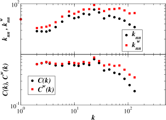
Figure 4: Assortativity and clustering for the North-American network. Circles correspond to topological quantities while squares are for affinity and weighted clustering.

II.4 Betweenness Centrality

A further characterization of the network is provided by considering quantities that takes into account the global topology of the network. For instance, the degree of a vertex is a local measure that gives a first indication of its centrality. However, a more global approach is needed in order to characterize the real importance of various nodes. Indeed, some particular low-degree vertices may be essential because they provide connections between otherwise separated parts of the network. In order to take properly into account such vertices, the betweenness centrality (BC) is commonly used freeman77 ; newman01 ; goh01 ; barthelemy:2003b . The betweenness centrality of a node $v$ is defined as

$$g(v)=\sum_{s\neq t}\frac{\sigma_{st}(v)}{\sigma_{st}}$$ (10)

where $\sigma_{st}$ is the number of shortest paths going from $s$ to $t$ and $\sigma_{st}(v)$ is the number of shortest paths going from $s$ to $t$ and passing through $v$. This definition means that central nodes are part of more shortest paths within the network than peripheral nodes. Moreover, the betweenness centrality gives in transport networks an estimate of the traffic handled by the vertices, assuming that the number of shortest paths is a zero-th order approximation to the frequency of use of a given node. It is generally useful to represent the average betweenness centrality for vertices of the same degree

$$g(k)=\frac{1}{N_{k}}\sum_{v/k_{v}=k}g(v)\ .$$ (11)

For most networks, $g(k)$ is strongly correlated with the degree $k$. In general, the largest the degree and the largest the centrality. For scale-free networks it has been shown that the centrality scales with $k$ as

$$g(k)\sim k^{\mu}$$ (12)

where $\mu$ depends on the network newman01 ; goh01 ; barthelemy:2003b . For some networks however, the BC fluctuations around the behavior given by Eq. (12) can be very large and “anomalies” can occur, in the sense that the variation of the centrality versus degree is not a monotonous function. Guimerà and Amaral amaral:2004 have shown that this is indeed the case for the air-transportation network. This is a very relevant observation in that very central cities may have a relatively low degree and vice versa. In Fig. 5 we report the average behavior along with the scattered plot of the betweenness versus degree of all airports of the North American network. Also in this case we find very large fluctuations with a behavior similar to those observed in Ref. amaral:2004 . Interestingly, Guimerà and Amaral have put forward a network model embedded in real space that considers geopolitical constraints. This model appears to reproduce the betweenness centrality features observed in the real network pointing out the importance of space as a relevant ingredient in the structure of networks. In the following we focus on the interplay between spatial embedding, topology and weights in a simple general model for weighted networks in order to provide a modeling framework considering these three aspects at once.

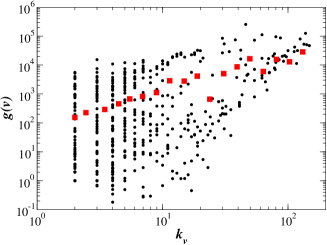
Figure 5: Scatter-plot of the betweenness centrality versus degree for nodes of the North-American air-transportation network. The red squares correspond to the average BC versus degree.

III The model

Early modeling of weighted networks just considered weight and topology as uncorrelated quantities yook:2001 . This is not the case in real world networks where a complex interplay between the evolution of weights and topological growth does exist. For instance, if a new airline connection between two airports is created, it will generally provoke a modification of the existing traffic of both airports. In general, it will increase the traffic activity depending on the specific nature of the network and on the local dynamics. This effect is introduced in the modeling of growing networks by the mechanism of a strength preferential attachment together with a dynamical redistribution of weights. Following this strategy it is possible to produce weighted networks with broad distributions of weights, connectivities, and strengths, and correlations between weights and topology barrat:2004b ; barrat:2004c .

Here we consider a weighted growing network whose nodes are embedded in a two-dimensional space. As in the weighted model of Ref. barrat:2004b , it is reasonable to think that a newly created node $n$ will establish links towards pre-existing nodes with heavy traffic or strength (hubs). Costs are however associated with distances and there is a trade-off between the need to reach a hub in a few hops and the connection costs. The cost naturally increases with the distance implying that the probability of establishing a connection between the new node $n$ and a given vertex $i$ decays as a function of the increasing Euclidean distance $d_{ni}$. As in the case of topological preferential attachment (i.e. connecting probability proportional to the degree barabasi:1999 ), this trade-off can be expressed in two different ways: the connecting probability can decrease either as a power-law of the distance manna02 ; xulvi02 ; yook02 or as an exponential with a finite typical scale barthelemy:2003a as it seems more natural for networks such as transportation networks (see Fig. 3) or technological networks waxman88 . All the effects described in the next paragraphs are obtained in the case of an exponential decay $\exp(-d_{ni}/r_{c})$ but are also present in the case of a power-law $d_{ni}^{-a}$ (the effect of a decreasing scale $r_{c}$ is qualitatively the same as the effect of an increasing exponent $a$). Eventually, the creation of new edges will introduce new traffic which will trigger perturbations in the network. This model therefore consists of two combined mechanisms:

1. Growth. We start with an initial seed of $N_{0}$ vertices randomly located (with uniform distribution) on a $2$-dimensional disk (of radius $L$) and connected by links with assigned weight $w_{0}$. At each time step, a new vertex $n$ is placed on the disk at a randomly assigned position ${\bf x}_{n}$ (still according to a uniform distribution). This new site is connected to $m$ previously existing vertices, choosing preferentially nearest sites with the largest strength. More precisely, a node $i$ is chosen according to the probability

   $$\Pi_{n\to i}=\frac{s_{i}^{w}e^{-d_{ni}/r_{c}}}{\sum_{j}s_{j}^{w}e^{-d_{nj}/r_{c}}},$$ (13)

   where $r_{c}$ is a typical scale and $d_{ni}$ is the Euclidean distance between $n$ and $i$. This rule of strength driven preferential attachment with spatial selection, generalizes the preferential attachment mechanism driven by the strength to spatial networks. Here, new vertices connect more likely to vertices which correspond to the best interplay between Euclidean distance and strength.

2. Weights dynamics. The weight of each new edge $(n,i)$ is fixed to a given value $w_{0}$ (this value sets a scale so we can take $w_{0}=1$). The creation of this edge will perturb the existing interactions and we consider local perturbations for which only the weights between $i$ and its neighbors $j\in{\cal V}(i)$ are modified

   $$w_{ij}\to w_{ij}+\delta\frac{w_{ij}}{s^{w}_{i}}.$$ (14)

After the weights have been updated, the growth process is iterated by introducing a new vertex, i.e. going back to step (1.) until the desired size of the network is reached.

The previous rules have simple physical and realistic interpretations. Equation (13) corresponds to the fact that new sites try to connect to existing vertices with the largest strength, with the constraint that the connection cannot be too costly. This adaptation of the rule “busy get busier” introduced in barrat:2004b ; barrat:2004c allows to take into account physical constraints. The weights’ dynamics Eq. (14) expresses the perturbation created by the addition of the new node and link. It yields a global increase of $w_{0}+\delta$ for the strength of $i$, which will therefore become even more attractive for future nodes.

The value of $\delta$ characterizes the susceptibility of the network. If $\delta<w_{0}$, the new link does not have a large influence. The case $\delta\approx w_{0}$ corresponds to situations for which the new created traffic (on the new link $n-i$) is transferred onto the already existing connections in a “conservative” way. Finally, $\delta>w_{0}$ is an extreme case in which a new edge generates a sort of multiplicative effect that is bursting the weight or traffic on neighbors.

The model contains two relevant parameters: the ratio between the typical scale and the size of the system $\eta=r_{c}/L$, and the ability to redistribute weights, $\delta$. Depending on the value of $\eta$ and $\delta$ we obtain different networks whose limiting cases are summarized in Figure 6. More precisely, we expect:

Figure 6: Different limiting regimes of the model depending on the value of its parameters $\delta$ and $\eta$.

• For $\eta\gg 1$, the effect of distance is negligible and we recover the properties of the weighted model of Ref. barrat:2004b . In this case, one obtains power-law distributions for connectivities and strengths with exponent $\gamma=(4\delta+3)/(2\delta+1)$, as well as for the weights (exponent $\alpha=2+1/\delta$). The strength and degree are linearly related by $s^{w}(k)\simeq(2\delta+1)k$. The effect of the redistribution parameter $\delta$ is to broaden the various probability distributions, and to increase the correlations between topology and weights. Moreover, no correlations are introduced between the topology of the network and the underlying two-dimensional space, so that the distance strength $s^{d}$ grows simply linearly with the degree.

• When $\eta$ decreases, additional constraints appear and have consequences that we will investigate numerically in the following. Unless otherwise specified, the simulations correspond to the parameters $m=3$ (i.e. an average degree $\langle k\rangle=6$), and $\delta=1.0$. We consider networks of size up to $N=10,000$, and the results are averaged over up to $100$ realizations. All the observed dependences in $\eta$ are essentially the same for other investigated values of $\delta$.

IV Numerical results

IV.1 Topology and weights

At a purely topological level, the principal effect of a typical finite scale $r_{c}$ in the creation of new connections is to introduce a cut-off in the scale-free degree distributions barthelemy:2003a . In Fig. 7 we report the degree distribution for a fixed value of $\delta$ and decreasing values $\eta$. A more pronounced cut-off appears at decreasing value of $\eta$ signalling the onset of a trade-off between the number of connections and their cost in terms of Euclidean distance. The small-world properties of the network are as-well modified barthelemy:2003a : on the one hand, the increasing tendency to establish connections in the geographical neighborhood favors the formation of cliques and leads to an increase in the clustering coefficient (see inset of Fig. 8). On the other hand, this same tendency leads to an increase in the diameter of the graph, measured as the average shortest path distances between pairs of nodes. The diameter however still increases logarithmically with the size of the graph, as shown in Fig. 8: the constructed networks do display the small-world property, even if strong geographical constraints are present.

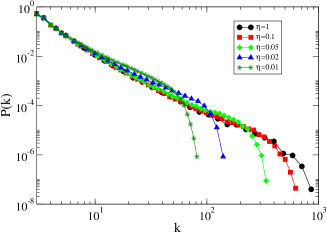
Figure 7: Degree distribution $P(k)$ for different values of $\eta$ and $\delta=1$. The degree distribution is averaged over $50$ networks of size $N=10^{4}$ and minimum degree $m=3$.

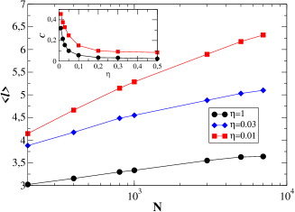
Figure 8: Average shortest path distances as a function of the network size $N$ for different values of $\eta$, with $m=3$ and $\delta=1$. Inset: clustering coefficient as a function of $\eta$ for $N=10^{4}$, $\delta=1$ (circles) and $\delta=5$ (squares). The data are averaged over $50$ networks.

The correlations appearing between traffic and topology of the network are presented in Fig. 9 for two extreme cases of large and small $\eta$. Strikingly, the effect of the spatial constraint is to increase both exponents $\beta_{w}$ and $\beta_{d}$ to values larger than $1$ and although the redistribution of the weights [Eq. (14)] is linear, non-linear relations $s^{w}(k)$ and $s^{d}(k)$ as a function of $k$ appear. For the weight strength the effect is not very pronounced with an exponent of order $\beta_{w}\approx 1.1$ for $\eta=0.01$, while for the distance strength the non-linearity has an exponent of order $\beta_{d}\approx 1.27$ for $\eta=0.02$ (the value of the exponents $\beta_{w}$ and $\beta_{d}$ depend on $\eta$; see also manna:2005 for a spatial model with $\beta_{d}>1$). We show on Fig. 9 the distance strength for two extreme situations for which spatial constraints are inexistent ($\eta=10.0$) or on the contrary very strong ($\eta=0.02$).

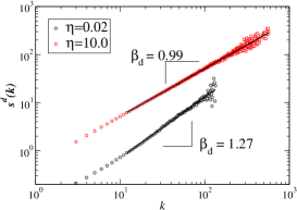
Figure 9: Distance strength versus $k$ for $\eta=0.02$ and $\eta=10.0$ (the networks are obtained for $\delta=1$, $N=10^{4}$, $\langle k\rangle=6$, and averaged over $100$ configurations). When $\eta$ is not small, space is irrelevant and there are no correlations between degree and space. When spatial effects are important ($\eta=0.02\ll 1$), non-linear correlations appear. We observe a crossover for $k\simeq 10-20$ to a power-law behavior and the power-law fit over this range of values of $k$ is shown (full lines).

The nonlinearity induced by the spatial structure can be explained by the following mechanism affecting the network growth. The increase of spatial constraints affects the trend to form global hubs, since long distance connections are less probable, and drives the topology towards the existence of “regional” hubs of smaller degree. The total traffic however is not changed with respect to the case $\eta=\infty$, and is in fact directed towards these “regional” hubs. These medium-large degree vertices therefore carry a much larger traffic than they would do if global “hubs” were available, leading to a faster increase of the traffic as a function of the degree, eventually resulting in a super-linear behavior. Moreover, as previously mentioned, the increase in distance costs implies that long range connections can be established only towards the hubs of the system: this effect naturally lead to a super-linear accumulation of $s^{d}(k)$ at larger degree values.

Spatial constraints have also a strong effect on the correlations between neighboring nodes (Fig. 10). At large $\eta$, a disassortative network is created, as is the case in most growing networks barrat:2004e ; as $\eta$ decreases, $k_{nn}$ decreases, and an increasing range of flat $k_{nn}(k)$ appears: the tendency for small nodes to connect to hubs is contrasted by the need to use small-range links. For small enough $\eta$, a nearly neutral behavior more similar to what is actually observed in the airport network is reached. Moreover, the affinity of nodes to establish strong links to large nodes, measured by $k_{nn}^{w}(k)$, goes from a flat behavior at large $\eta$ to a slightly assortative one at small $\eta$. In all cases, the weighted correlation $k_{nn}^{w}(k)$ remains clearly larger than the unweighted $k_{nn}(k)$, showing that links to busier nodes are typically stronger.

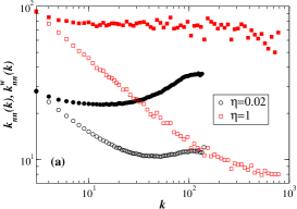
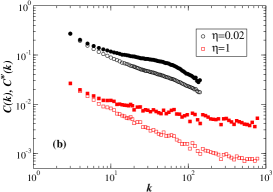
Figure 10: (a) Assortativity and (b) clustering versus $k$ obtained for the model for $\delta=1$, $N=10^{4}$, $\langle k\rangle=6$, $\eta=0.02$ (circles) and $\eta=1$ (squares). Data are averaged over $100$ configurations. Empty symbols refer to topological correlations while full symbols correspond to the weighted quantities $k_{nn}^{w}$ and $C^{w}$.

A non-trivial clustering hierarchy is already displayed by the model without spatial constraints. As previously mentioned, the decrease of $\eta$ leads to an increase of clustering. Moreover, the weighted clustering is always significantly larger than the unweighted one, showing that the cliques carry typically an important traffic (see Fig. 10). These effects are a general signature of spatial constraints as also observed in a non weighted network barthelemy:2003a .

IV.2 Spatial constraints and betweenness centrality

The spatial constraints act at both local and global level of the network structure by introducing a distance cost in the establishment of connections. It is therefore important to look at the effect of space in global topological quantities such as the betweenness centrality. The betweenness centrality of a vertex is determined by its ability to provide a path between separated regions of the network. Hubs are natural crossroads for paths and it is natural to observe a marked correlation between $g$ and $k$ as expressed in the general relation $g(k)\sim k^{\mu}$. The exponent $\mu$ depends on the characteristics of the network and we expect this relation to be altered when spatial constraints become important. In the present model, Fig. 11 clearly shows that this correlation in fact increases when spatial constraints become large (i.e. when $\eta$ decreases). This can be understood simply by the fact that the probability to establish far-reaching short-cuts decreases exponentially in Eq. (13) and only the large traffic of hubs can compensate this decay. Far-away geographical regions can thus only be linked by edges connected to large degree vertices, which implies a more central role for these hubs.

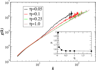
Figure 11: Betweenness centrality versus degree for different values of $\eta$. Inset: Exponent $\mu$ (obtained by fitting the data for $k>10$) of the betweenness centrality versus $\eta$ (for $N=5,000$, $m=3$ and averaged over $50$ configurations). For strong spatial constraints long-range shortcuts are very rare and hubs connect regions which are otherwise almost disconnected which in turn implies a larger centrality of the hubs.

Figure 12: (a) Betweenness centrality for the (one-dimensional) lattice case. The central nodes are close to the barycenter. (b) For a general graph, the central nodes are usually the ones with large degree.

In order to better understand the effect of space on the properties of betweenness centrality, we have to explicitly consider the geometry of the network along with the topology. In particular, we need to consider the role of the spatial position by introducing the spatial barycenter of the network. Indeed, in the presence of a spatial structure, the centrality of nodes is correlated with their position with respect to the barycenter $G$, whose location is given by ${\bf x}_{G}=\sum_{i}{\bf x}_{i}/N$. For a spatially ordered network—the simplest case being a lattice embedded in a one-dimensional space—the shortest path between two nodes is simply the Euclidean geodesic. In a limited region, for two points lying far away, the probability that the shortest path passes near the barycenter of all nodes is very large. In other words, this implies that the barycenter (and its neighbors) will have a large centrality. In a purely topological network with no underlying geography, this consideration does not apply anymore and the full randomness and the disordered small world structure are completely uncorrelated with the spatial position. It is worth remarking that the present argument applies in the absence of periodic boundary conditions that would destroy the geometrical ordering. This point is illustrated in Fig. 12 in the simple case of a one-dimensional lattice.

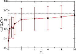
Figure 13: Average Euclidean distance between the barycenter $G$ of all nodes and the $10$ most central nodes ($C$) versus the parameter $\eta$ (Here $\delta=0$, $N=5,000$ and the results are averaged over $50$ configurations). When space is important (ie. small $\eta$), the central nodes are closer to the gravity center. For large $\eta$, space is irrelevant and the average distance tends to the value corresponding to a uniform distribution $\langle r\rangle_{unif}=2/3$ (dotted line).

The present model defines an intermediate situation in that we have a random network with space constraints that introduces a local structure since short distance connections are favored. Shortcuts and long distance hops are present along with a spatial local structure that clusters spatially neighboring vertices. In Fig. 13 we plot the average distance $d(G,C)$ between the barycenter $G$ and the $10$ most central nodes. As expected, as spatial constraints become more important, the most central nodes get closer to the spatial barycenter of the network.

Another effect observed when the spatial constraints become important are the large fluctuations of the BC. Fig. 14a displays the relative fluctuation

$$\delta g(k)=\frac{\sqrt{\langle\delta g^{2}(k)\rangle}}{\langle g(k)\rangle}\,,$$ (15)

where $\langle\delta g^{2}(k)\rangle$ is the variance of the BC and $\langle g(k)\rangle$ its average (computed for each value of $k$). The value of $\eta$ modifies the degree cut-off and in order to be able to compare the results for different values of $\eta$ we rescale the abscissa by its maximum value $k_{max}$. This plot (Fig. 14a) clearly shows that the BC relative fluctuations increase as $\eta$ decreases and become quite large. This means that nodes with small degree may have a relatively large BC (or the opposite), as observed in the air-transportation network (see Fig. 5 and amaral:2004 ). In order to quantify these “anomalies” we compute the fluctuations of the betweenness centrality $\Delta_{RN}(k)$ for a randomized network with the same degree distribution than the original network and constructed with the Molloy-Reed algorithm molloyreed . We consider a node $i$ as being “anomalous” if its betweenness centrality $g(i)$ lies outside the interval $[\langle g(k)\rangle-\alpha\Delta_{RN}(k),\langle g(k)\rangle+\alpha\Delta_{RN}(k)]$, where we choose $\alpha\simeq 1.952$ so that the considered interval would represent $95\%$ of the nodes in the case of Gaussian distributed centralities around the average.

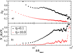
Figure 14: (a) Relative fluctuations of the betweenness centrality versus $k/k_{max}$ for two values of $\eta$ ($N=5,000$ and the results are averaged over $50$ configurations and binned). The fluctuations increase when $\eta$ decreases (i.e. when spatial constraints increase). (b) Number of anomalies $N_{a}(k)$ rescaled by the number of nodes $N_{k}$ versus $k/k_{max}$ for different values of $\eta$. The relative number of anomalies is larger when spatial constraints are large, especially for large $k$.

In Fig. 14b, we show the relative number of anomalies versus $k/k_{kmax}$ for different values of $\eta$. This plot shows that the relative number of anomalies $N_{a}(k)/N_{k}$ increases when the degree increases and more interestingly strongly increases when $\eta$ decreases. Note that since for increasing $k$ the number of nodes $N_{k}$ is getting small, the results become more noisy.

The results of Figs. (11-14) can be summarized as follows. In a purely topological growing network, centrality is strongly correlated with degree since hubs have a natural ability to provide connections between otherwise separated regions or neighborhoods barthelemy:2003b . As spatial constraints appear and become more important, two factors compete in determining the most central nodes: (i) on the one hand hubs become even more important in terms of centrality since only a large traffic can compensate for the cost of long-range connections which implies that the correlations between degree and centrality become thus even stronger; (ii) on the other hand, many paths go through the neighborhood of the barycenter, reinforcing the centrality of less-connected nodes that happen to be in the right place; this yields larger fluctuations of $g$ and a larger number of “anomalies”.

We finally note that these effects are not qualitatively affected by the weight structure and we observe the same behavior for $\delta=0$ or $\delta\neq 0$.

V Conclusions

In this paper, we have presented a model of growing weighted networks introducing the effect of space and geometry in the establishment of new connections. When spatial constraints appear, the effects on the network structure can be summarized as follows:

• (i) Effect of spatial embedding on topology-traffic correlations
  Spatial constraints induce strong nonlinear correlations between topology and traffic. The reason for this behavior is that spatial constraints favor the formation of regional hubs and reinforces locally the preferential attachment, leading for a given degree to a larger strength than the one observed without spatial constraints. Moreover, long-distance links can connect only to hubs, which yields a value $\beta_{d}>1$ for small enough $\eta$. The existence of constraints such as spatial distance selection induces some strong correlations between topology (degree) and non-topological quantities such as weights or distances.

• (ii) Effect of space embedding on centrality
  Spatial constraints also induce large betweenness centrality fluctuations. While hubs are usually very central, when space is important central nodes tend to get closer to the gravity center of all points. Correlations between spatial position and centrality compete with the usual correlations between degree and centrality, leading to the observed large fluctuations of centrality at fixed degree.

• (iii) Effect of space embedding on clustering and assortativity
  Spatial constraints implies that the tendency to connect to hubs is limited by the need to use small-range links. This explains the almost flat behavior observed for the assortativity. Connection costs also favor the formation of cliques between spatially close nodes and thus increase the clustering coefficient.

Including spatial effects in a simple model of weighted networks thus yields a large variety of behavior and interesting effects. This study sheds some light on the importance and effect of different ingredients such as spatial embedding or diversity of interaction weights in the structure of large complex networks and we believe that this attempt of a network typology could be useful in the understanding and modeling of real-world networks.

- (1) R. Albert and A.-L. Barabási, Rev. Mod. Phys. 74, 47 (2002).
- (2) S.N. Dorogovtsev and J.F.F. Mendes, Adv. Phys. 51, 1079 (2002).
- (3) S. N. Dorogovtsev and J. F. F. Mendes, Evolution of networks: From biological nets to the Internet and WWW (Oxford University Press, Oxford, 2003).
- (4) R. Pastor-Satorras and A. Vespignani, Evolution and structure of the Internet: A statistical physics approach (Cambridge University Press, Cambridge, 2004).
- (5) R. Cohen, K. Erez, D. ben Avraham, and S. Havlin, Phys. Rev. Lett. 85, 4626 (2000).
- (6) D.S. Callaway, M.E.J. Newman, S.H. Strogatz,, and D.J. Watts, Phys. Rev. Lett. 85, 5468 (2000).
- (7) R. Albert, H. Jeong, and A.-L. Barabási, Nature 406, 378 (2000).
- (8) R. Pastor-Satorras and A. Vespignani, Phys. Rev. Lett. 86, 3200 (2001).
- (9) A.E. Krause, K. A. Frank, D. M. Mason, R. E. Ulanowicz, and W. W. Taylor, Nature 426, 282 (2003).
- (10) M. Granovetter, American Journal of Sociology, 78 (6) 1360-1380 (1973).
- (11) D. Garlaschelli, S. Battiston, M. Castri, V.D.P. Servedio, and G. Caldarelli, Physica A 350, 491 (2005).
- (12) W. Li and X. Cai, Phys. Rev. E 69, 046106 (2004).
- (13) C. Li and G. Chen, Preprint cond-mat/0311333 (2003).
- (14) A. Barrat, M. Barthélemy, R. Pastor-Satorras, and A. Vespignani, Proc. Natl. Acad. Sci. USA 101, 3747 (2004).
- (15) E. Almaas, B. Kovács, T. Viscek, Z.N. Oltval and A.L. Barabási, Nature 427, 839 (2004).
- (16) A. Helmy, online archive: cs.NI/0207069.
- (17) G. Nemeth and G. Vattay, Phys. Rev. E 67, 036110 (2003).
- (18) S.P. Gorman and R. Kulkarni, submitted to Environment and Planning Journal B, (2003).
- (19) M.T. Gastner and M.E.J. Newman, condmat/0407680
- (20) M.T. Gastner and M.E.J. Newman, condmat/0409702
- (21) A. Lakhina, J.B. Byers, M. Crovella, and I. Matta, technical report, online version available at : http://www.cs.bu.edu/techreports/pdf/2002-015-internet-geography.pdf
- (22) M. Barthélemy, Europhys. Lett. 63, 915 (2003).
- (23) R. Guimerà and L.A.N. Amaral, Eur. Phys. J. B 38, 381 (2004).
- (24) A. Barrat, M. Barthélemy, and A. Vespignani, Phys. Rev. Lett., 92, 228701 (2004).
- (25) A. Barrat, M. Barthélemy, and A. Vespignani, Phys. Rev. E 70 (2004) 066149.
- (26) A. Barrat, M. Barthélemy, and A. Vespignani, LNCS 3243 (2004) 56.
- (27) R.V.R. Pandya. Preprint cond-mat/0406644 (2004).
- (28) S.N. Dorogovtsev and J.F.F. Mendes, preprint cond-mat/0408343.
- (29) T. Antal and P.L. Krapivsky, Preprint cond-mat/0408285.
- (30) G. Bianconi, Power-law strength-connectivity dependence in weighted scale-free networks, cond-mat/0412399.
- (31) W.-X. Wang, B. Hu, G. Yan, Q. Ou and B.-H. Wang, Interplay of dynamics, traffic and topology on technological networks, preprint cond-mat/0501215.
- (32) R. Guimerà, S. Mossa, A. Turtschi, and L.A.N. Amaral, Preprint cond-mat/0312535 (2003).
- (33) L.A.N. Amaral, A. Scala, M. Barthélemy, and H.E. Stanley, Proc. Natl. Acad. Sci. (USA) 97, 11149 (2000).
- (34) http://www.iata.org.
- (35) S.H. Yook, H. Jeong, A.-L. Barabasi, and Y. Tu, Phys. Rev. Lett. 86, 5835 (2001).
- (36) A. Vázquez, R. Pastor-Satorras and A. Vespignani, Phys. Rev. E 65, 066130 (2002).
- (37) M. E. J. Newman, Phys. Rev. Lett. 89, 208701 (2002).
- (38) D. J. Watts and S. H. Strogatz, Nature 393, 440–442 (1998).
- (39) J.-P. Onnela, J. Saramäki, J. Kertész, K. Kaski, cond-mat/0408629.
- (40) L. C. Freeman, Sociometry 40, 35 (1977) .
- (41) K.-I. Goh, B. Kahng, and D. Kim, Phys. Rev. Lett. 87, 278701 (2001) .
- (42) M. E. J. Newman, Phys. Rev. E 64, 016131 (2001); Phys. Rev. E 64, 016132 (2001).
- (43) M. Barthélemy, Eur. Phys. J. B 38, 163 (2003).
- (44) A.-L. Barabasi and R. Albert, Science 286, 509 (1999).
- (45) S.S. Manna and P. Sen Phys. Rev. E 66, 066114 (2002).
- (46) R. Xulvi-Brunet and I.M. Sokolov, Phys. Rev. E 66, 026118 (2002).
- (47) S.-H. Yook, H. Jeong, and A.-L. Barabasi, Proc. Natl. Acad. Sci. (USA) 99, 13382 (2002).
- (48) B.M. Waxman, IEEE J. Select. Areas. Commun. 6, 1617 (1988).
- (49) G. Mukherjee and S. S. Manna, cond-mat/0503697.
- (50) A. Barrat and R. Pastor-Satorras, Phys. Rev. E 71, 036127 (2005).
- (51) M. Molloy and B. Reed, Random Struct. Algorithms 6, 161 (1995).