Hamilton’s principle: why is the integrated difference of kinetic and potential energy minimized?

Abstract

I present an intuitive answer to an often asked question: why is the integrated difference $K-U$ between the kinetic and potential energy the quantity to be minimized in Hamilton’s principle? Using elementary arguments, I map the problem of finding the path of a moving particle connecting two points to that of finding the minimum potential energy of a static string. The mapping implies that the configuration of a non–stretchable string of variable tension corresponds to the spatial path dictated by the Principle of Least Action; that of a stretchable string in space-time is the one dictated by Hamilton’s principle. This correspondence provides the answer to the question above: while a downward force curves the trajectory of a particle in the $(x,t)$ plane downward, an upward force of the same magnitude stretches the string to the same configuration $x(t)$.

I Introduction

Nature loves extremes. Soap films seek to minimize their surface area and adopt a spherical shape; a large piece of matter tends to maximize the gravitational attraction between its parts and, as a result, planets are also spherical; light rays refracting on a magnifying glass bend and follow the path of least time, and a relativistic particle chooses to follow the path between two events in space-time that maximizes the time measured by a clock on the particle.taylor1 ; foot0 Nor are humans divorced from extremum principles, attempting to reduce the complexities of the world to the smallest number of dominating principles.

For mechanical systems, this goal has been accomplished by Maupertuis and Hamilton in different versions of the celebrated Principle of Least Action. Both formulations emerge from conceiving the trajectories of particles as light rays traversing different media which, according to Fermat, follow the path that minimizes time.

In 1744, Maupertuis proposed that “Nature, in the production of its effects, does so always by the simplest means” maupertuis1 and, in 1746, wrote “in Nature, the action (la quantité d’action) necessary for change is the smallest possible. Action is the product of the mass of a body times its velocity times the distance it moves”.maupertuis2 For a light ray or a particle passing from one medium into another, both the minimization of time and minimization of action gives rise to angles of incidence and refraction in a fixed proportion to each other: the analog of Snel’s lawsnel for a light ray $n_{1}\sin\theta_{1}=n_{2}\sin\theta_{2}$ corresponds to the conservation of particle momentum along the interface $mv_{1}\sin\theta_{1}=mv_{2}\sin\theta_{2}$. Even though Maupertuis’ formulation was vague–and there was controversy on the priority over the ideamaupertuis3 –his name remains attached to the principle arguably for two reasons: his metaphysical view that minimum action expresses God’s wisdom in the form of an economy principleterrall , and Euler’s role in settling the controversy in his favor.

Hamilton’s principle, formulated almost a century later, is similar to the Principle of Least Action and is based on the optical-mechanical analogy as well.hamilton While the trajectory followed by a particle of fixed energy $E$ connecting two points in space is prescribed by the Principle of Least Action, Hamilton’s principle determines the trajectory for which the particle will spend a given time $t$ in travelling between the same points. In such a case, the optimal path is the one for which the sum of the products $(K-U)\Delta t$ along the path is a minimum ($K$ and $U$ are the kinetic and potential energies and $\Delta t$ the time interval). Hamilton’s method was mentioned throughout the nineteenth century but was rarely used in practice because simpler methods were as effective in most cases.hamilton1

The situation changed in 1926 when Schrödinger, inspired by de Broglie’s ideas, resorted to Hamilton’s analogy between mechanics and geometric optics, extended the treatment from geometrical to undulatory mechanics, and arrived at his famous equation for the dynamics of a quantum mechanical particle.schrodinger Moreover, in 1948, Feynmanfeynman (following a hint from Dirac) offered a new perspective on Hamilton’s principle: in propagating between two points, a quantum particle “explores” every path, treating them on equal footing. This “democracy of histories”mtw becomes the Principle of Least Action for a classical particle due to destructive interference that eliminates those paths that differ significantly from the classical (or extremal) path.

A lesser known approach to what is called now the Principle of Least Action was taken by John Bernoullibernoulli , who showed that Snel’s law can be obtained from the condition of mechanical equilibrium of a tense, non-stretchable string (see Figure 1). This analogy was also noted by Möbiusmobius0 ; mobius and discussed by Ernst Mach in his classical book on mechanics.mach Ref. cebreros considers an inextensible string and is the only article I was able to find on this analogy.

In the present paper I show that a simple extension of this idea to paths that are covered in fixed time can be used to prove the equivalence of Hamilton’s principle to the static equilibrium of a stretchable string. My aim is to provide, in the spirit of References hanc ; moore ; hanc2 ; hanc3 ; hanc4 , insight into why it is the the difference between the kinetic and potential energy that appears in Hamilton’s principle. In section II, I review Bernoulli’s approach and in section III, I present a simplified derivation of Hamilton’s principle without calculus. In section IV, I present a slightly more elaborate derivation using elementary calculus. Given the importance of the Principle of Least Action in so many areas of Physics, I hope that this paper will contribute to its presentation in introductory courses rather than it being postponed to advanced mechanics courses.

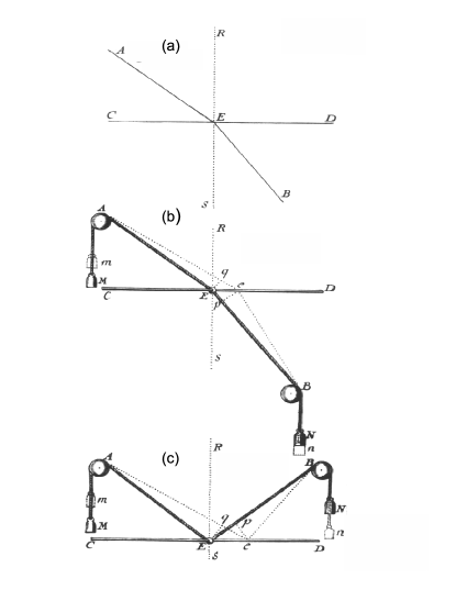
Figure 1: (a) and (b) John Bernoulli’s proof of Snel’s law using the mechanical equilibrium of a tense string. (c) Mechanical model for the law of reflection, which is not discussed in the present paper. (Figure reproduced from Reference bernoulli ).

II The Least Action Principle and non-stretchable strings

Figure 1 shows the diagram used by John Bernoulli to derive Snel’s law for a light ray travelling from point $A$ to $B$ using the analogy with the static equilibrium of a tense string. The following is a rephrasing of Bernoulli’s argument, which is based on the hypothesis that, in mechanical equilibrium, it is equivalent to say that the net force on each point of the system is zero, and that the system is in the state of minimum potential energy. In discussing the particle motion I will assume knowledge of Newton’s law $\textbf{F}=\Delta\textbf{p}/\Delta t$ relating the force on a particle with the rate of chance of its momentum.

Call $T_{1}$ and $T_{2}$ the weights hanging from points $A$ and $B$; the point of contact between the upper and lower portions of the string slides horizontally without friction along the line $CD$. The pulleys at $A$ and $B$ are considered frictionless and with zero inertia; therefore the tensions of the different portions of the string will be $T_{1}$ and $T_{2}$. Compare the potential energy of the configurations where the point of contact are $E$ and $e$. There is a potential energy difference between the two configurations because in going from $E$ to $e$, mass 1 will rise from $M$ to $m$ and mass 2 will decrease its height from $N$ to $n$. The tensions are determined by the weights and are, therefore, in both configurations, $T_{1}$ and $T_{2}$. Calling $\ell_{1}=AE$ and $\ell_{2}=EB$, the change in potential energy $\Delta U$ of the system becomes

$$\Delta U=T_{1}\Delta\ell_{1}+T_{2}\Delta\ell_{2},$$ (1)

where $\Delta\ell_{1}=Mm\equiv qe$ and $\Delta\ell_{2}=-Nn\equiv Ep$. This means that, up to an additive constant, the potential energy of the system can be written as

$$U=T_{1}\ell_{1}+T_{2}\ell_{2}.$$ (2)

Another way of visualizing the above expression is offered in Figure 2.

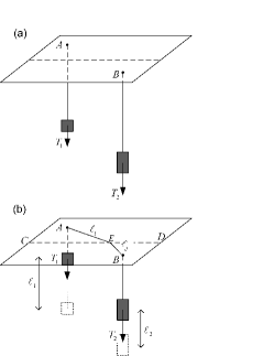
Figure 2: An alternative version of Bernoulli’s setup: (a) Two weights hanging from frictionless points $A$ and $B$ is assigned zero potential energy. (b) The two weights are then lifted, and the ends of the strings are joined at point $E$ along the line $CD$. The work done is equal to the increase in potential energy: $U=T_{1}\ell_{1}+T_{2}\ell_{2}$.

Since the configuration of mechanical equilibrium corresponds to the minimum of potential energy the minimum $U$ is attained when the components of the forces from the different portions of the string along $CD$ cancel. In term of the angles $\angle AER=\theta_{1}$ , $\angle SEB=\theta_{2}$, the minimum potential energy is attained when

$$T_{1}\sin\theta_{1}=T_{2}\sin\theta_{2}.$$ (3)

The above relation is equivalent to Snel’s law if the indices of refraction $n_{1}$ and $n_{2}$ in the different regions are identified with the corresponding tension of the strings: if the time $t$ is minimized, or equivalently the optical length $ct$ given by

$$ct=n_{1}\ell_{1}+n_{2}\ell_{2},$$ (4)

then $n_{1}\sin\theta_{1}=n_{2}\sin\theta_{2}$. For the analogy between the configuration of the tense string and the trajectory of a particle with energy $E$ between points $A$ and $B$ I reason in reverse: knowing that conservation of momentum at the interface requires

$$mv_{1}\sin\theta_{1}=mv_{2}\sin\theta_{2},$$ (5)

what is the magnitude that should be minimized in order to get the above relation? Clearly, from the above analysis the quantity to be minimized is

$$A=mv_{1}\ell_{1}+mv_{2}\ell_{2},$$ (6)

which is Maupertuis’ action. The correspondence between Eq. 4 and Eq. 6 expresses the famous analogy between mechanics and geometric optics that has been the subject of many recent pedagogical expositionsfma ; pform .

The tension $T_{i}$ of the string is identified with the velocity $v_{i}$ on each region which, in turn, is given by $v_{i}=\sqrt{2m(E-U_{i})}$, where $E$ is the total energy and $U_{i}$ is the corresponding potential energy. For paths that transverse many regions where the particle velocities are different, the trajectory has to be broken up in many straight segments. The Principle of Least Action states that the trajectory the particle will follow between two fixed points and at fixed total energy is the one that minimizes the sum of the products $mv_{i}\ell_{i}$ in each segment. In order to use the analogy with the string, the arrangement will correspond to frictionless pulleys that can slide on rods, with the string passing through them a sufficient number of timesmach (see Figure 3).

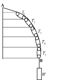
Figure 3: Frictionless pulleys that can slide in horizontal lines with a string passing through them a sufficient number of times gives the trajectory of the particle if $T_{i}$ is identified with $mv_{i}$ at each segment. Since the string can only pass through each pulley an integer number of times, the ratios of the velocities are approximated by the ratio of the times the rope passes through each segment.

Table 1 summarizes the analogies between the quantities discussed in this section.

Table 1: Corresponding quantities in the analogy used in the Principle of Least Action between mechanics, geometric optics and the equilibrium of a non-stretchable string.

Particle	Light Ray	Non-stretchable string
$mv$ (momentum)	$n$ (refractive index)	$T$ (tension)
$mv_{1}\sin\theta_{1}=mv_{2}\sin\theta_{2}$ (momentum conservation)	$n_{1}\sin\theta_{1}=n_{2}\sin\theta_{2}$ (Snel’s law)	$T_{1}\sin\theta_{1}=T_{2}\sin\theta_{2}$ (static equilibrium)
$\Delta A=mv\Delta\ell$ (action)	$c\Delta t=n\Delta\ell$ (optical length)	$\Delta U=T\Delta\ell$ (potential energy)

III Hamilton’s principle and stretchable strings

The Principle of Least Action as stated in the previous paragraph gives the optimal trajectory for a particle of a given energy between two fixed points. It doesn’t say anything about the time it takes to travel from one point to the other. Now consider the problem of finding a path that will connect point $P$ to point $Q$ in a fixed time $t$. In other words, what is the path that the particle will choose in going from point ${\rm{\bf P}}=(x_{P},0)$ to point ${\rm{\bf{Q}}}=(x_{Q},t)$? In extending the treatment to paths that go from two fixed space–time points it is useful to treat $t$ as a new geometrical dimension. To simplify the analysis, and to retain the two dimensional picture of the previous paragraph, I will consider motion in one (spatial) dimension.

Consider the path as a continuous function $x(t)$, that is broken into small straight segments connecting points separated by a fixed time interval $\Delta t$. The fact that the segments are straight means that the motion is of constant velocity during that interval, then changes due to an impulsive force. This force will be different from zero if the potential is changing as a function of $x$ at the particle position. Consider for simplicity two broken segments as in Figure 4(a).

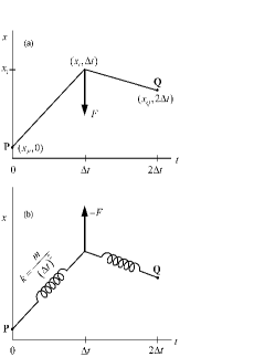
Figure 4: (a) Space-time trajectory of an otherwise free one-dimensional particle acted upon by an impulsive force $F$ at $t_{i}=\Delta t$. (b) Equivalent equilibrium configuration of two segments of a stretchable string with spring constants $k=m/(\Delta t)^{2}$ and an external force $-F$.

Before the force $F$ acts on the particle, the velocity is given by the slope of the curve in the $(x,t)$ plot:

$$v_{P}={x_{i}-x_{P}\over\Delta t}.$$ (7)

The effect of the force is to change the velocity. In the $(x,t)$ plot (also called the “world line”), this means that the slope of the line changes at the intermediate time. The velocity after the force has acted on the particle is

$$v_{Q}={x_{Q}-x_{i}\over\Delta t}.$$ (8)

Notice that, since the force is downward, the slope decreases: downward force means that, at $x_{i}$ , the potential is increasing as a function of $x$.

The path [in space time $(x,t)$] is a solution of Newton’s second law, according to which the rate of change of the velocity times the particle mass is the force acting on it:

$$F=m{v_{Q}-v_{P}\over\Delta t}.$$ (9)

Replacing the above expressions for the velocity:

$$F={m\over\left(\Delta t\right)^{2}}\left(x_{Q}-x_{i}\right)-{m\over\left(\Delta t\right)^{2}}\left(x_{i}-x_{P}\right).$$ (10)

At this point take a step of abstraction, and forget the space-time picture for a moment. This expression gives the force of a system of two springs of identical spring constant, the first spring connecting point $(x_{i},\Delta t)$ with $(x_{P},0)$, the second connecting $(x_{Q},2\Delta t)$ with $(x_{i},\Delta t)$. In order for the systems to be in equilibrium, or, in other words, for the intermediate coordinate to have the value $x_{i}$ (the other two are fixed) there has to be a force of precisely magnitude $F$ but of opposite sign.

The path given by Newton’s law is given by the equilibrium condition of a mechanical model of two springs in the presence of a potential of opposite sign as $U(x)$. The equilibrium condition is the one that minimizes the potential energy of the entire system, springs plus “external” potential $U(x)$. Since the potential energy for a spring of spring constant $k$ connecting two points separated by a distance $\delta$ is $k\delta^{2}/2$ , the total potential energy of the system (that I will call $\widetilde{S}$) is given by

$$\widetilde{S}={m\over 2}\left({x_{i}-x_{P}\over\Delta t}\right)^{2}+{m\over 2}\left({x_{Q}-x_{i}\over\Delta t}\right)^{2}-U(x_{i}).$$ (11)

Coming back to the original world line picture, the optimum path in space–time is the one that minimizes the difference between kinetic and potential energy. This is Hamilton’s principle, which I obtained using a mechanical analogy similar to the Principle of Least Action in the sense that there is a correspondence between the kinetic energy and the potential energy of fictitious springs of spring constant $k=m/(\Delta t)^{2}$. In other words, the stretchable string is in equilibrium due to two types of forces in space-time: the external force due to (minus) the real external potential, and the elastic force of fictitious springs playing the role of the kinetic energy.

For a a longer path with $N$ straight segments each of them traversed by the particle in a time $\Delta t$, the velocity at the $i$-th segment will be $v_{i}=(x_{i+1}-x_{i})/\Delta t$ and the equivalent potential energy will be given by

$$\widetilde{S}=\left[{mv_{1}^{2}\over 2}-U(x_{1})\right]+\left[{mv_{2}^{2}\over 2}-U(x_{2})\right]+\cdots+{mv_{N}^{2}\over 2}.$$ (12)

For a large number of segments, which will correspond to a continuously varying path, the last term in the sum above can be ignored; the total potential energy to be minimized is the sum of the differences between the kinetic and potential energies.

Notice that the potential energy for the fictitious springs corresponds to springs of zero length. Also, Equations 11 and 12 omit the potential energy associated with the “horizontal displacement” $\Delta t$ of each spring. I ignore this contribution because the horizontal forces due to the springs cancel and, therefore, the potential energy associated with this displacement is the same for all configurations of the string.

IV Hamilton’s principle using elementary calculus

IV.1 Connection between Maupertuis’ and Hamilton’s action

In this section I, derive Hamilton’s principle using a slightly more sophisticated approach while still keeping it elementary. In reference to Figure 1(a), the Principle of Least Action tells us the path a particle of fixed energy $E$ will choose in going from $A$ to $B$. Call $U_{1}$ and $U_{2}$ the potential energies in the upper and lower parts of the line $CD$, and $v_{1}=\sqrt{2m(E-U_{1})}$ and $v_{2}=\sqrt{2m(E-U_{2})}$ the corresponding velocities. Now consider paths with different energies and ask for which of those paths the particle will satisfy Newton’s laws and spend a fixed amount of time $t$ going from $A$ to $B$. Following the logic of the Principle of Least action, I want to find a function of the paths that will give the desired one upon minimization. For the special case in consideration, the path consists of two straight segments and the function has to be such that, of all paths that take a time $t$ in going from $A$ to $B$, it chooses the one that satisfies the “Snel’s law for particles” of Eq. 5.

Call $a$ and $b$ the perpendicular distances of $A$ and $B$ to the interface $CD$, $L$ the horizontal distance between $A$ and $B$ and $x$ the distance $CE$. Maupertius action of Eq. 6 can be thought of as a function of $x$ and the energy:

$$A(x,E)=mv_{1}(E)\sqrt{x^{2}+a^{2}}+mv_{2}(E)\sqrt{(L-x)^{2}+a^{2}}.$$ (13)

In order to explore whether $A(x,E)$ is the desired function, compute the variations of $A$ with respect to $x$ and $E$, assuming knowledge of the ratios of $dE$ and $dx$ that will keep the time $t$ constant:

$$dA=\left(mv_{1}\sin\theta_{1}-mv_{2}\sin\theta_{2}\right)dx+{\partial A\over\partial E}dE.$$ (14)

It is clear that minimizing $A$ (or equivalently setting $dA=0$) does not give us the desired Eq.5 because of the second term above. However, notice that $dv_{i}/dE=1/mv_{i}$, and

$${\partial A\over\partial E}={\sqrt{x^{2}+a^{2}}\over v_{1}}+{\sqrt{(L-x)^{2}+a^{2}}\over v_{2}}=t_{1}+t_{2}=t,$$ (15)

with $t_{1}\equiv\ell_{1}/v_{1}$ and $t_{2}\equiv\ell_{2}/v_{2}$ the times it takes the particle to go from $A$ to $B$ and from $E$ to $B$.

This means that if $Et$ is subtracted from $A$ the desired quantity is obtained: $S=A-Et$. (Notice that $d(Et)=tdE$ since the paths considered last a constant time.) Therefore,

$$S = \left(mv_{1}\ell_{1}-Et_{1}\right)+\left(mv_{2}\ell_{1}-Et_{2}\right)$$ (16)

$$= \left(mv_{1}^{2}-E\right)t_{1}+\left(mv_{2}^{2}-E\right)t_{2}$$

$$= \left(K_{1}-U_{1}\right)t_{1}+\left(K_{2}-U_{2}\right)t_{2},$$

which is the quantity to be minimized according to Hamilton’s principle.

IV.2 Could Hamilton have discovered quantum mechanics in 1834?

Writing $p=mv$ and $\ell=x$, the above action $S$ (Eq.16) for a path has precisely the form of the phase change of a wave

$$\phi\sim px-Et$$ (17)

(up to a multiplicative constant that will render it dimension-less) with momentum and energy playing the role of wave number $k$ and frequency $\omega$. The path of least–or, more precisely stationary–action could hence be regarded as the stationary phase limit of some wave. With this motivation I ask wether Hamilton could have discovered quantum mechanics in 1834. The answer is most probably “no,” since Hamilton did not have any experimental motivation to think of particles as waves.hamilton0 However, the close parallelism between geometric optics and mechanics could have invited him to ask himself the following: what would be the structure of a wave equation for particles that, in the limit of small wavelengths, gives the trajectories of particles just as the wave equation for light in the same limit gives the trajectories of light rays?

Let us follow the analogy provided by the Principle of Least Action and consider trajectories of constant energy for particles which will correspond to light rays of constant frequency. Since the Principle of Least Action establishes an equivalence between the geometry of trajectories and not between the dynamics of those trajectories, for constant energy (and frequency) I seek an equivalence between stationary states of the corresponding wave equations.

Now let us introduce wave-lengths into the discussion. The wave length of a monochromatic light wave in a region in which the index of refraction $n(x)$ is varying slowly is given by

$$\lambda(x)={\lambda_{0}\over n(x)}.$$ (18)

Since equations 4 and 6 imply that the trajectories of particles and light rays are equivalent if $n(x)$ is identified with $mv(x)$, the “natural” choice for the spatial dependence of the particle wave length $\lambda_{P}$ is

$$\lambda_{P}(x)={K\over mv(x)}={K\over\sqrt{2m\left[E-U(x)\right]}},$$ (19)

with $K$ a constant that has units of angular momentum and is precisely the required constant to make $\phi$ in Eq. 17 dimension-less: $\phi={2\pi\over K}(px-Et)$.

Now let us consider the wave equation for the amplitude $\phi(x,t)$ describing a light wave in one dimension (I ignore the polarization and consider it as a scalar wave)foot1 :

$${\partial^{2}\phi\over\partial x^{2}}={n^{2}(x)\over c^{2}}{\partial^{2}\phi\over\partial t^{2}}.$$ (20)

I want to compare this with the stationary wave equation for particles, so I substitute $\phi(x,t)=\phi(x)e^{i\omega t}$

and the equation becomes

$$-\left({\lambda_{0}\over 2\pi}\right)^{2}{\partial^{2}\phi\over\partial x^{2}}=n^{2}(x)\phi.$$ (21)

Using the equivalences of Eqs. 18 and 19, the structure of the wave equation for the stationary states $\Psi$ for particles should be

$$-{\left(K/2\pi\right)^{2}\over 2m}{\partial^{2}\Psi\over\partial x^{2}}=\left[E-U(x)\right]\Psi.$$ (22)

In comparison with Eq. 21, if $K$ is treated as a free parameter, the limit $K\rightarrow 0$ (which corresponds to the limit $\lambda_{0}\rightarrow 0$) gives the trajectories for particles of energy $E$ and Eq. 22 could be used as a wave equation for particles. If many years later someone were to discover that particles in confined potentials had discrete energies, $K$ could be tuned to fit the experiments obtaining

$${K\over 2\pi}=1.0546\times 10^{-34}{\rm J\,s},$$ (23)

which is of course Planck’s constant $\hbar$. Given the identification of energy with frequency, the time dependence of the stationary states should be $\Psi(x)e^{-iEt/\hbar}$ and the “naturally” implied time dependence for Eq. 22 is

$$\left[-{\hbar^{2}\over 2m}{\partial^{2}\over\partial x^{2}}+U(x)\right]\Psi=i\hbar{\partial\over\partial t}\Psi,$$ (24)

which is the celebrated Schrödinger equation.

V conclusion

I have presented an elementary derivation of Hamilton’s principle based on the analogy between particle (and light ray) trajectories with the configuration of a tense non-stretchable string. The analogy was (to my knowledge) first considered by Bernoulli in a practically unreferenced article and gives an intuitive picture of the Principle of Least Action. Extending the analogy to stretchable strings, I derived Hamilton’s principle, providing an intuitive picture of the origin of the difference between kinetic and potential energy in Hamilton’s characteristic function. I also presented a derivation using elementary calculus, which extends the analogy between mechanics and geometrical optics to undulatory mechanics and “derived” Schrödinger’s equation.

I have endeavored to present a pedagogical approach that can help students in introductory courses appreciate the beauty and compactness of the Principle of Least Action.

- (1) E. F. Taylor and J. A. Wheeler, Exploring Black Holes, 1st edition (Addison Wesley, San Francisco, 2000), Chap. 1, p.5.
- (2) Strictly speaking, extremal (maxima or minima) are a subset stationary paths (or states). However, the term Principle of Least Action is more frequently used than the more precise Principle of Stationary Action.
- (3) P. L. Moreau de Maupertuis, “Accord de différentes loix de la nature, qui avaient jusqu’ici paru incompatible,” Memoires de l’Académie Royale de Sciences (Paris) pp. 417-26 (1744), reprinted in Oeuvres, 4 pp. 1-23 Reprografischer Nachdruck der Ausg. Lyon (1768).
- (4) P. L. Moreau de Maupertuis, “Recherche des lois du Mouvement”, Reprinted Oeuvres, 4 p. 36.
- (5) The English spelling (Snell) found in most textbooks of the name of the Dutch astronomer and mathematician Willebrord Snel (1580-1626) derives from its Latinized version Willebrodus Snellius. See for example K. Hentschel, “The law of refraction according to Snellius - Reconstruction of his path of discovery and a translation of his Latin manuscript along with additional documents”, Arch. Hist. Exact. Sci. 55, pp. 297-344 (2001).
- (6) Several years before, Clairaut [in “Sur les explications Cartésienne et Newtonienne de la réfraction de la lumière”, Memoires de l’Académie Royale de Sciences (Paris) pp. 259-75 (1739)] had shown that Newtonian attraction could be applied to refraction. The controversy with Samuel Koenig, who accused Maupertuis of plagiarizing Gottfried Wilhelm Leibniz’s work in this principle is detailed in P. Brunet, Etude Historique sur le Principe de La Moindre Action, Herman & Cie, Éditeurs, Paris, 1938.
- (7) See for example M. Terrall, The Man Who Flattened the Earth, Maupertuis and the Sciences of Enlightenment (The University of Chicago Press, Chicago, 2002) pp. 178-179.
- (8) W. R. Hamilton, “On a general method of expressing the paths of light, and of the planets, by the coefficients of a characteristic function,” Dublin University Review and Quarterly Magazine, 1, 795-826 (1833).
- (9) For a historical account see T. L. Hankins, Sir William Rowan Hamilton, (The John Hopkins University Press, Baltimore, 1980).
- (10) E. Schrödinger, Collected Papers on Wave Mechanics (Blackie & Son Limited, London 1928), pp. 13-27.
- (11) R. P. Feynman, “Space-Time Approach to Non-relativistic Quantum Mechanics,” Rev. Mod. Phys., 20, pp. 367-387 (1948).
- (12) The phrase is taken from C. W. Meisner, K. S. Thorne and J. A. Wheeler, Gravitation (W. H. Freeman and Company, New York, 1973) pp. 499-500.
- (13) J. Bernoulli, “Disquisitio Catoptico-Dioptrica,” Opera Omnia, (Geneve, sumptibus Marci-Michaelis Bousquet & sociorum, 1742) Vol. 1, pp. 369-376.
- (14) A. F. Möbius, Lehrbuch der Statik, Sweiter Theil. (Liepzig, 1837) pp. 217-313.
- (15) J. Gray, “Möbius’s geometrical mechanics,” included in Möbius and his band edited by J. Fauvel, R. Flood and R. Wilson (Oxford University Press, Oxford, 1993) pp.79-103.
- (16) E. Mach, The Science of Mechanics: Account of its Development, translated by Thomas J. McCormack, sixth edition, (The Open Court Publishing Company, Illinois, 1960) pp. 463-474.
- (17) C. Bellver-Cebreros and M. Rodriguez-Danta, “Eikonal equation from continuum mechanics and analogy between equilibrium of a string and geometrical light rays,” Am. J. Phys. 69, 360-367 (2001).
- (18) J. Hanc, S. Tuleja and M. Hancova, “Simple derivation of Newtonian mechanics from the principle of least action,” Am. J. Phys. 71, 386-391 (2004).
- (19) T. A. Moore, “Getting the most action out of least action: A proposal,” Am. J. Phys. 72, 522-527 (2004).
- (20) J. Hanc and E. F. Taylor, “From conservation of energy to the principle of least action: A story line,” Am. J. Phys. 72, 514-521 (2004).
- (21) J. Hanc, E. F. Taylor and S. Tuleja “ Deriving Lagrange’s equations using elementary calculus,” Am. J. Phys. 72, 510-513 (2004).
- (22) J. Hanc, E. F. Taylor and S. Tuleja “ Variarional mechanics in one and two dimensions,” Am. J. Phys., in press.
- (23) J. Evans and M. Rosenquist, “ ‘F=ma’ optics,” Am. J. Phs 54, 876-883 (1986).
- (24) D. S. Lemons, Perfect Form (Princeton University Press, Princeton 1997).
- (25) In consonance with this historical excercise it could be objected that Hamilton didn’t know the wave equation for light, but the argument applies to any scalar wave in a nonhomogeneous medium. For example, Eq. 20 could represent a sound wave in a medium with varying density.
- (26) The title of this section was taken from Ref.hamilton1 p. 209.