Hausdorff clustering of financial time series

Abstract

A clustering procedure, based on the Hausdorff distance, is introduced and tested on the financial time series of the Dow Jones Industrial Average (DJIA) index.

, , , ,

1 Introduction

Clustering consists in grouping a set of objects in classes according to their degree of “similarity” [1]. This intuitive concept can be defined in a number of different ways, leading in general to different partitions. For this reason, it is clear that a clustering procedure can be profoundly influenced by the strategy adopted by the observer and his/her own ideas and preconceptions about the data set. In this article we will focus on a linkage algorithm, that consists in merging, at each step, the two clusters with the smallest dissimilarity, starting from clusters made up of a single element and ending up in a single cluster collecting all data. Our objective will be to cluster the financial time series of the stocks belonging to the Dow Jones Industrial Average (DJIA) index.

From a mathematical point of view, given a set of objects $\mathcal{S}\equiv\{s\}$, an allocation function $m:\mathcal{S}\rightarrow\{1,2,\dots,k\}$, is defined so that $m(s)$ is the class label and k the total number of clusters (which we assume to be finite for simplicity). The aim of a clustering procedure is to select, among all possible allocation functions, the one performing the best partition of the set ${\mathcal{S}}$ into subsets $\mathcal{G}_{\alpha}\equiv\{s\in\mathcal{S}|m(s)=\alpha\},(\alpha=1,\dots,k)$, relying on some measure of similarity.

Clustering algorithms can be classified in different ways according to the criteria used to implement them. The so-called “hierarchical” methods yield nested partitions, represented by dendrograms [2], in which any cluster can be further divided in order to observe its underlying structure. Linkage algorithms, in particular, are hierarchical. Other non-hierarchical (or “partitional”) methods are also possible [3, 4, 5], but will not be discussed here.

2 Hausdorff clustering

In order to cluster a given data set we will use a distance function introduced by Hausdorff. Given a metric space $({\mathcal{S}},\delta)$, with metric $\delta$, the distance between a point $a\in{\mathcal{S}}$ and a subset $B\subseteq{\mathcal{S}}$ is naturally given by

$$\tilde{d}(a;B)=\inf_{b\in B}\delta(a,b)$$ (1)

(all subsets are henceforth considered to be non-empty and compact). Given a subset $A\subseteq{\mathcal{S}}$, let us define the function

$$\tilde{d}(A;B)=\sup_{a\in A}\tilde{d}(a;B)=\sup_{a\in A}\inf_{b\in B}\delta(a,b),$$ (2)

which measures the largest among all distances $\tilde{d}(a;B)$, with $a\in A$. This function is not symmetric, $\tilde{d}(A;B)\neq\tilde{d}(B;A)$, and therefore is not a bona fide distance. The Hausdorff distance [6] between two sets $A,B\subseteq{\mathcal{S}}$ is defined as the largest between the two numbers:

$$d_{\rm H}(A,B) = \max\{\tilde{d}(A;B),\tilde{d}(B;A)\}$$ (3)

$$= {\max}\{\sup_{a\in A}\inf_{b\in B}\delta(a,b),\sup_{b\in B}\inf_{a\in A}\delta(a,b)\}$$

and is clearly symmetric.

In words, the Hausdorff distance between $A$ and $B$ is the smallest positive number $r$, such that every point of $A$ is within distance $r$ of some point of $B$, and every point of $B$ is within distance $r$ of some point of $A$. The meaning of the Hausdorff distance is best understood by looking at an example, such as that in Fig. 1. We emphasize that the Hausdorff metric relies on the metric $\delta$ on ${\mathcal{S}}$.

If the data set is finite and consists of $N$ elements, all distances can be arranged in a $N\times N$ matrix $\delta_{ij}$ and Eq. (3) reads

$$d_{\rm H}(A,B)=\max\{\max_{i\in A}\min_{j\in B}\delta_{ij}~{},\max_{j\in B}\min_{i\in A}\delta_{ij}\},$$ (4)

which is a very handy expression, as it amounts to finding the minimum distance in each row (column) of the distance matrix, then the maximum among the minima. The two numbers are finally compared and the largest one is the Hausdorff distance. This sorting algorithm is easily implemented in a computer.

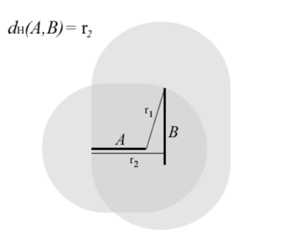
Figure 1: Hausdorff distance between two sets $A$ and $B$ (black thick segments). $r_{1}=\tilde{d}(B;A)$, $r_{2}=\tilde{d}(A;B)$. The Hausdorff distance is equal to the larger radius $r_{2}$.

The Hausdorff distance naturally translates in a linkage algorithm. At the first level each element is a cluster and the Hausdorff distance between any pair of points reads

$$d_{\rm H}(\{i\},\{j\})=\delta_{ij}$$ (5)

and coincides with the underlying metric.

The two elements of ${\mathcal{S}}$ at the shortest distance are joined together in a single cluster. The Hausdorff distance matrix is recomputed, considering the two joined elements as a single set. This iterative process goes on until all points belong to a single final cluster.

3 Comparison with single and complete linkage

It is interesting to notice that the partitions obtained by the Haudorff linkage algorithm are intermediate between those obtained by the more commonly used “single” and “complete” linkage procedures: if $A$ and $B$ are two non empty subsets of ${\mathcal{S}}$, the single and complete linkage algorithms make use of the following similarity indexes

$$d_{\rm S}(A,B) = \inf_{a\in A,b\in B}\delta(a,b),$$ (6)

$$d_{\rm C}(A,B) = \sup_{a\in A,b\in B}\delta(a,b),$$ (7)

respectively.

In order to compare these different algorithms, it is useful to recall the mathematical definition of distance. Given a set ${\mathcal{S}}$, a distance (or a metric) $\delta$ is a non-negative application

$$d:{\mathcal{S}}\times{\mathcal{S}}\longrightarrow\mathbb{R},$$ (8)

endowed with the following properties, valid $\forall x,y\in{\mathcal{S}}$:

$$d(x,y)=0\quad\Longleftrightarrow\quad x=y,$$ (9)

$$d(x,y)=d(y,x),$$ (10)

$$d(x,y)\leq d(x,z)+d(y,z),\quad\forall z\in{\mathcal{S}}.$$ (11)

Incidentally, notice that symmetry (10), as well as non-negativity, are not independent assumptions, but easily follow from (9) and the triangular inequality (11).

It is not difficult to prove from the very definition (3) that the Hausdorff distance between compact and non-empty sets satisfies (9)-(11). On the other hand, (6) and (7) are not distances: the former does not satisfy the triangular inequality (11), while the latter does not fulfil the basic requirement (9), $d_{\rm C}(A,A)\neq 0$, for any compact set containing more than one point: in this sense, it performs a sort of coarse graining over the data set. The Haussdorf function, being a distance in a strict mathematical sense, enables us to rest on sound mathematical ground.

The Hausdorff distance has never been used (to the best of our knowledge) in the context of clustering. It is a useful tool in the analysis of complex sets, with complicated (and even fractal-like) structures. It is in such a case that one expects that Hausdorff behave better than the other methods, since it relies on rigorous mathematical concepts.

4 Application to Financial Data

We now apply the Hausdorff linkage algorithm to a topic of growing interest: the analysis of financial time series. In particular, we focus on the $N=30$ shares composing the DJIA index, collecting the daily closure prices of its stocks for a period of 5 years (1998-2002). We chose this index for two reasons. First, because these data are easily accessible. The second, and more important reason is the “quality” (in the sense of reliability) of prices. The DJIA index, indeed, aggregates the shares of some of the more valuable and capitalized world corporations, so that their prices are highly contributed by market makers. This means that we always expect to find, even in the worst possible scenario, a financial intermediator (market maker) ready to quote both bid and offer prices for these assets. For this reason, these shares are very frequently traded. In financial terminology, they are said to be “liquid.”

Figure 2 displays the typical behavior of a stock value (IBM) for the investigated time period. The companies of the DJIA stock market are reported in Figure 3 (bottom right), together with the corresponding industries.

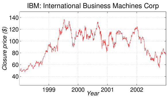
Figure 2: Time evolution of the closure price of a stock value (IBM), for the period 1998-2002.

We will look at the temporal series of the daily logarithm closure price differences

$$Y_{i}(t)\equiv\ln P_{i}(t)-\ln P_{i}(t-1),$$ (12)

where $P_{i}(t)$ is the closure price of the $i$th share at day $t$. Both $P_{i}$ and $Y_{i}$ are very irregular functions of time. In order to quantify the degree of similarity between two time series and use our linkage algorithm we adopt the following metric function, that quantifies the synchronicity in their time evolution [7, 8, 9]

$$d_{ij}=\sqrt{2(1-c_{ij})}~{},$$ (13)

where $c_{ij}$ are the correlation coefficients computed over the investigated time period:

$$c_{ij}=\frac{\langle Y_{i}Y_{j}\rangle-\langle Y_{i}\rangle\langle Y_{j}\rangle}{\sqrt{(\langle Y_{i}^{2}\rangle-\langle Y_{i}\rangle^{2})(\langle Y_{j}^{2}\rangle-\langle Y_{j}\rangle^{2})}}$$ (14)

and the brackets denote the average over the time interval of interest (one year in our case). Table 1 displays a part of the $N\times N$ matrix of the correlation coefficients (year 1998). It is worth stressing that almost all correlation coefficients are positive, with values not too close to 1, thus confirming that, in many cases, stocks belonging to the same market do not move independently from each other, but rather share a similar temporal behavior. The distance (13) is a proper metric in the “parent” space, ranging from 0 for perfectly correlated series ($c_{ij}=+1$) to 2 for anticorrelated stocks ($c_{ij}=-1$). (The representative points lie therefore on a hypersphere.)

	AA	AXP	BA	CAT	C
AA	1	0.37004	0.22458	0.3568	0.3508
AXP		1	0.35461	0.41916	0.61247
BA			1	0.32852	0.26917
CAT				1	0.33937
C					1

Table 1: A part of the matrix of the correlation coefficients $c_{ij}$ (14) for the temporal series of the daily logarithm price differences of the stocks composing the DJIA index (year 1998). The acronyms (tickers) are explained in Figure 3.

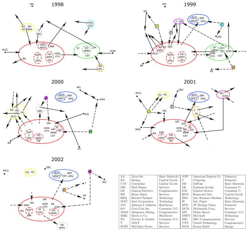
Figure 3: Clusters obtained by analyzing the daily logarithm closure price difference time series during 1998-2002. The innermost subclusters are indicated with a dashed bubble. Dashed arrows = past; full arrows = future. The position of the points representing the stocks is not directly related to the distance matrix (13) and has no effective “spatial” meaning: the pictorial representation simply reflects the aggregation of points and subclusters into larger clusters. Bottom right: acronyms (tickers) of the stocks and related industries (C. = Cyclical; N.C. = Non-Cyclical; Intl. = International)

5 Results and Discussion

Figure 3 shows the results of our analysis based on the Hausdorff ansatz. Rather than showing the dendrograms, we prefer to give a pictorial representation of the evolution of the stocks by using bubbles to represent clusters and arrows to represent the movements of the stocks. Some innermost subclusters are indicated with a dashed bubble and full (dashed) arrows denote future (past) movements. A small “exploding” star represents a bubble/cluster that disappears.

It is very interesting and challenging to try and analyze, from a mere economic viewpoint, some of the movements in the graphs, in order to catch some “a posteriori” hints about the dynamics of the stocks. At first sight, one clearly recognizes that some of the clusters correspond to homogeneous groups of companies belonging to the same industry: this is the case of the financial services firms {AXP, JPM  C}, retail companies {HD, WMT}, companies dealing with basic materials (AA, IP, DD), the technological core {IBM, INTC, MSFT, HPQ} and the health care firms {JNJ, MRK}.

Moreover, one observes a large super-cluster made up of 10-15 stocks (financial, conglomerates, services, capital goods), containing some homogenous subclusters, which is more or less stable during the whole 5-year period investigated.

It is worth stressing, between 1998 and 1999, the migration of the hi-tech companies {IBM, INTC, MSFT} from this cluster. At the end of these two years, they end up forming a separated cluster with HPQ, that remains stable for all the following period. As is well known, 1999 is the year when the high-tech bubble started to grow up. Even more interesting is the “path” of Disney. During 1998 it is perceived to be linked to HP, which was (and still is) its favorite supplier of hardware. Then, during the following years, it remains more or less single, until, between 2001 and 2002, it rejoins HP into the high-tech core. This evolution can probably be explained by remembering Disney’s strategic efforts to increase its Media Network segment, that consisted also in a series of acquisitions (the last two: Fox Family Worldwide Inc. and Baby Einstein Co).

We emphasize that these remarks are not an input of our analysis: our clustering algorithm is purely mathematical, and no genuinely “economical” information (e.g., on industrial homogeneity) was used at the outset. In this sense the position and movements of the stocks in the figures are implied from the market itself.

The definition of the mutual positioning of companies can have an immediate pertinence in a matter of great interest for financial institutions: the portfolio optimization. In a few words (and without entering into complex matters), portfolio theory suggests that in order to minimize the risk involved in a financial investment, one should diversify among different assets by choosing those stocks whose price time evolutions are as diverse as possible (it is never safe to put all the eggs into a single basket). Moreover, this strategy must be continuously updated, by changing weights and components, in order to follow the market evolution. In the framework we presented, by investigating the shares’ behavior and tracking the evolution of their mutual interactions, a first, crude portfolio-optimization rule that emerges would be: choose stocks belonging to clusters that are as “distant” as possible from each other.

In conclusion, we have introduced a novel clustering procedure based on the Hausdorff distance between sets. This genuinely mathematical method was used to investigate the time evolution of the stocks belonging to the DJIA index. We found the resulting partitions through the 5-year period investigated to be significant from an economical viewpoint and suited to a meaningful a posteriori analysis and interpretation. We believe that this technique is able to extract relevant information from the raw market data and yield meaningful hints for the investigation of the mutual time evolution of the stocks. For the same reasons this procedure could be implemented as the first step towards an evolved portfolio selection and optimization procedure.

Acknowledgements. We thank Sabrina Diomede for a discussion and a pertinent remark.

References

- [1] K. Fukunaga, Introduction to Statistical Pattern Recognition (Academic Press, San Diego, 1990).
- [2] A. K. Jain and R. C. Dubes, Algorithms for Clustering Data (Prentice Hall, New York, 1988).
- [3] A. Gersho and R. M. Gray, Vector Quantization and Signal Processing (Kluwer Academic Publisher, Boston, 1992).
- [4] R. O. Duda, P. E. Hart and D. G. Stork, Pattern Classification (John Wiley & Sons, New York, 2002).
- [5] T. Hofmann and J. M. Buhmann, Pairwise Data Clustering by Deterministic Annealing, IEEE Transaction on Pattern Analysis and Machine Intelligence, 19, 1 (1997).
- [6] F. Hausdorff, Grundzüge der Mengenlehre (von Veit, Leipzig, 1914). [Republished as Set Theory, 5th ed. (Chelsea, New York, 2001).]
- [7] R. N. Mantegna, Eur. Phys. J. B 11, 193 (1999).
- [8] R. N. Mantegna and H. E. Stanley, Introduction to Econophysics (Cambridge University Press, 2000).
- [9] M. Bernaschi, L. Grilli and D. Vergni, Physica A 308, 381 (2002); L. Grilli, Physica A 332, 441 (2004).