Autocatalytic reaction fronts between reacted and unreacted species may propagate as solitary waves, namely at a constant front velocity and with a stationary concentration profile, resulting from a balance between molecular diffusion and chemical reaction. A velocity field in the supporting medium may affect the propagation of such fronts through different phenomena: convection, diffusion enhancement, front shape changes… We report here on an experimental study and lattice BGK numerical simulations of the effect of an oscillating flow on the autocatalytic reaction between iodate and arsenous acid in a Hele-Shaw cell. In the low frequency range covered by the experiments, the front behavior is controlled by the flow across the gap and can be reproduced with 2D numerical simulations. An analytical solution is also derived under the condition of a weak flow velocity, and is found to be in reasonable agreement with our data.

Introduction

Interface motion and reaction front propagation occur in a number of different areas [1], including flame propagation in combustion [2], population dynamics [3, 4] and atmospheric chemistry (ozone hole). An autocatalytic reaction front between two reacting species propagates as a solitary wave, that is, at a constant front velocity and with a stationary front profile [5, 6]. These issues were addressed earlier on, but only a few cases are understood, such as the pioneering works of Fisher [3] and Kolmogorov-Petrovskii-Piskunov [4] on a reaction-diffusion equation with a second-order kinetics [1, 7, 8]. Although the effect of an underlying flow on a flame propagation has been extensively analyzed [2, 7], the advective effect on the behavior of an autocatalytic front has been addressed only recently [9, 10, 11, 12]. In this case, the evolution of the concentration of each chemical species is given by the Advection-Diffusion-Reaction (ADR) equation:

$$\frac{\partial C}{\partial t}+\overrightarrow{U}.\overrightarrow{\triangledown}C=D_{m}\triangle C+\alpha f(C)$$ (1)

where $C$ is the normalized concentration of the (autocatalytic) reactant, $\overrightarrow{U}$ is the flow velocity, $D_{m}$ is the molecular diffusion coefficient and $\alpha$ is the reaction rate.
In the absence of flow ($\overrightarrow{U}=\overrightarrow{0}$), the balance between diffusion and reaction leads to a solitary wave of constant velocity $V_{\chi}$ and width $l_{\chi}$. For the autocatalytic Iodate-Arsenous Acid (IAA) reaction studied here, the kinetics is of the third order [1], $f(C)=C^{2}(1-C)$, and the following $1D$ solution of equation (1) is obtained [6, 13]:

$$C(z,t)=\frac{1}{1+e^{(z-V_{\chi}t)/l_{\chi}}}\;\;,\;\;l_{\chi}=\sqrt{\frac{2D_{m}}{\alpha}}\;\;,\;\;V_{\chi}=\sqrt{\frac{\alpha D_{m}}{2}}$$ (2)

where $z$ is the direction of the front propagation.

For a reaction propagating along the direction of a unidirectional stationary flow, $\overrightarrow{U}$, two regimes have been described, depending on the ratio $\eta=b/2l_{\chi}$, where $b$ is the typical length scale transversely to the flow direction [14, 15, 16]. In the eikonal regime, $\eta\gg 1$, the front propagates as a planar wave, at a velocity given by the sum of $V_{\chi}$ and of the algebraic maximum of the flow velocity (projected onto the direction of $\overrightarrow{V_{\chi}}$), and takes the according stationary form. In the mixing regime, $\eta\ll 1$, the interplay between diffusion and advection enhances the mixing of the chemical species and leads to an overall macroscopic diffusion known as Taylor hydrodynamic dispersion [17]. As a result, the front moves faster. However, it is still described by equation (2), in which the molecular diffusion coefficient $D_{m}$ has to be replaced by its effective macroscopic counterpart.

The main idea of the present paper is to address the effect of an unsteady flow on the front propagation. We measure, experimentally and numerically, the velocity and width of a chemical front submitted to a time periodic flow, of period $T=1/f=2\pi/\omega$. The question of the relevant time scale, to which the time scale of the flow, $T$, has to be compared, is discussed.

We extend the theoretical work by Nolen and Xin et al. [12], who derived the time-averaged chemical front velocity in an oscillating flow, by analyzing the temporal evolution of the front velocity. We note that in the tracer case (without reaction), Chatwin [18] and Smith [19] showed, using a Taylor-like approach [17], that a pulsating flow results in an effective time dependent diffusion coefficient, the time-average of which is larger than the molecular diffusion coefficient [20].

In this paper, we study, experimentally and numerically, a third-order autocatalytic Iodate-Arsenous Acid (IAA) reaction submitted to a pulsative flow. In section $1$, we present the experimental set-up and the measurements obtained using a large set of frequencies and amplitudes of oscillations. In section $2$, we compare the experimental results with $2D$ numerical simulations and we investigate a wider range of parameters with additional simulations. In the last section, we extend the theoretical result by Nolen and Xin [12] to derive the temporal variations of the front velocity.

Experimental set-up and data

We use the third-order autocatalytic Iodate-Arsenous Acid (IAA) reaction. The reaction front is detected with starch, leading to a dark blue signature of the transient iodine as the reaction occurs [1, 6, 13]. In the absence of flow, a reaction front travels like a solitary wave, with a constant velocity $V_{\chi}^{exp}\sim 20\;\mu m/s$ and with a stationary concentration profile of width $l_{\chi}^{exp}\sim 100\;\mu m$. We study the front propagation in a Hele-Shaw (HS) cell of cross-section $b\times h=0.4\times 8\;mm^{2}$ (along $x$ and $y$ directions, respectively). The unidirectional (along $z$ direction) oscillating flow is imposed at the bottom of a vertical HS cell, from a reservoir filled with unreacted species. This revervoir is closed with a thin elastic membrane, pressed in its middle by a rigid rod fixed at the center of a loudspeaker. Consequently, a displacement of a given volume of liquid in the reservoir induces a displacement of the same volume of liquid in the HS cell. The $y-z$ plane of the HS cell is enlightened from behind and recorded with a CCD camera. The amplitude $A$ and the pulsation $\omega=2\pi f$ of the oscillating flow are imposed by the controlled sine tension applied to the loudspeaker, and measured in situ, from the recorded displacement of the air/liquid interface at the top of the partially filled HS cell. This displacement follows the expected $A\sin{(\omega t)}$ time dependence. Due to the constraint of our device, the imposed amplitude and frequency of the flow displacement are in the ranges $A\in[0.07\;mm,1.7\;mm]$ and $f\in[0.01\;Hz,0.2\;Hz]$ and the maximum velocity of the flow in the cell is roughly $U_{M}=A\omega$. The oscillating flow field in the HS cell is of the form (see Appendix for the full expression):

$$U(x,y,t)=U_{M}\Re e[f(x,y)]\sin{(\omega t)}$$ (3)

The shape of the velocity profile depends drastically on the viscous penetration length $l_{\nu}=\sqrt{\nu/\omega}$ [21]. If $l_{\nu}$ is large compared to the cell thickness $b$ (low frequency), the flow variations are slow enough for the steady state to be established. The resulting ”oscillating stationary” velocity profile is parabolic in the gap and flat along the width $h$ of the cell except in the vicinity of the side walls, in a layer of thickness $b$ [22]. Conversely, for $l_{\nu}<<b$ (high frequency), the fluid has not enough time to feel the effects of the solid boundaries and the velocity profile is flat over the whole cross-section $b\times h$, except in the vicinity of each wall, in a layer of thickness $l_{\nu}$. Figure 1 is a sketch of such an effect. For our dilute aqueous solutions of viscosity $\nu\approx 10^{-6}\;m^{2}.s^{-1}$ and in our frequency range, the penetration length $l_{\nu}$, which ranges between $0.8\;mm$ and $4\;mm$, is larger than the cell thickness $b=0.4\;mm$.

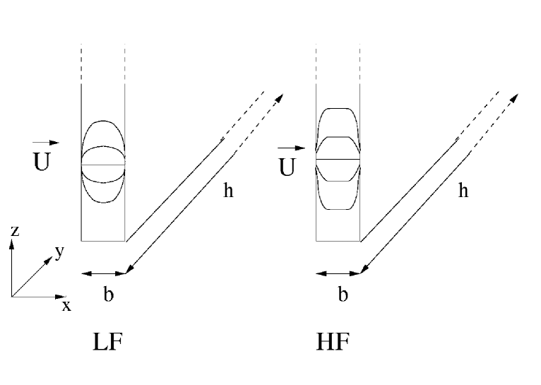
Figure 1: Sketch of the velocity profile in the gap of a Hele-Shaw cell for low frequency (LF, left) and high frequency (HF, right).

Hence, in most of our experiments, the ”stationary velocity profile” is instantaneously reached, parabolic Poiseuille-like across the gap $b$, and almost invariant along the $y$ direction (except in a layer of thickness $l_{\nu}$ close to the boundaries).

Figure 2 displays snapshots of a typical experiment: We do observe a front slightly deformed, propagating up and down (oscillating), with a downward averaged displacement, from the burnt product of the reaction to the fresh reactant.

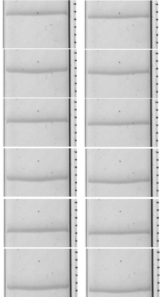
Figure 2: Time evolution of a chemical front in a pulsative flow field of amplitude $A=0.55\;mm$ and period $T=50\;s$. Time increases from left to right and from top to bottom. Two images are separated by $T/4$ time intervals. The distance between two dashes is $1\;mm$.

From this movie, the front is tracked and its location is plotted as a function of time. The so-obtained figure 3 clearly shows the oscillation of the front position at roughly the imposed frequency and an overall drift of the front.

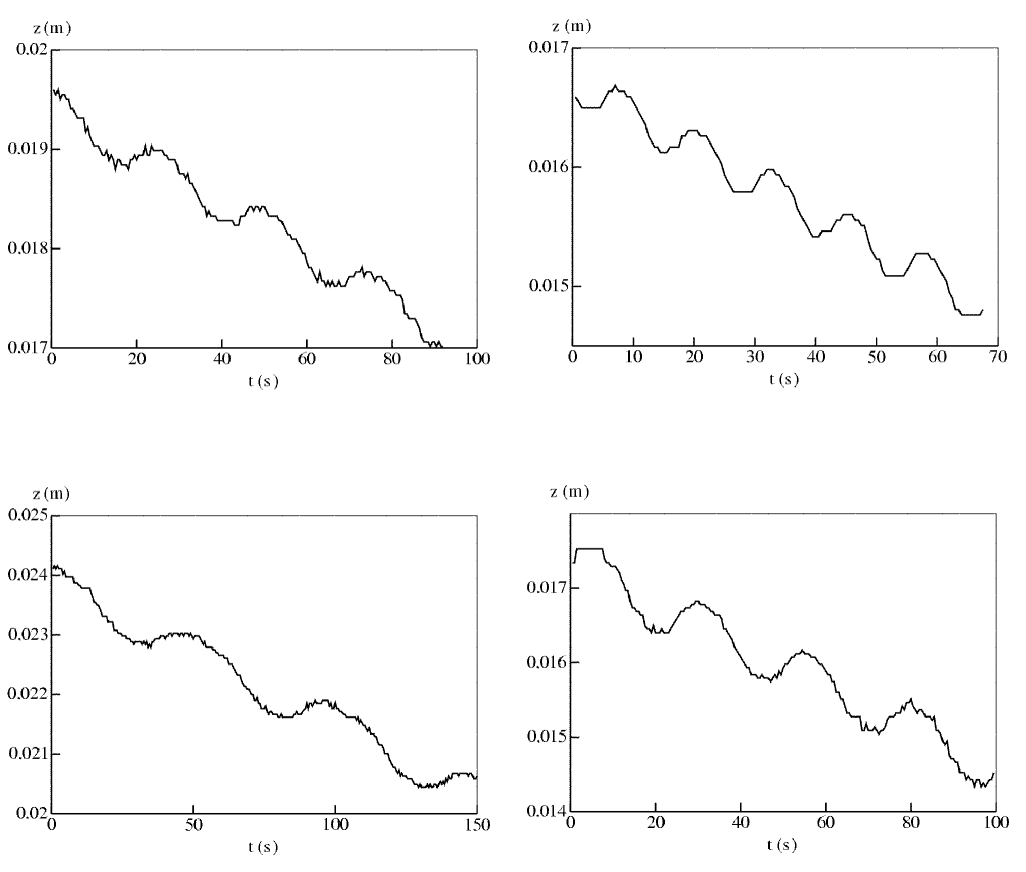
Figure 3: Front displacement for different couples $(A,f)$ ($A$ in $mm$ and $f$ in $Hz$). Top : $(0.28,0.04)$, $(0.55,0.02)$. Bottom : $(0.28,0.08)$, $(0.55,0.04)$.

The measurement of this drift in time leads to the time-averaged front velocity $\langle V_{f}^{exp}\rangle$. Figure 4 displays $\langle V_{f}^{exp}\rangle$, normalized by $V_{\chi}^{exp}$, versus the amplitude of the time-periodic flow field $\overline{U}=2U_{M}/3=2A\omega/3$ (where $2/3$ is the ratio of the gap-averaged velocity to the maximum one of a $2D$ gap Poiseuille profile), also normalized by $V_{\chi}^{exp}$. The increase of $\langle V_{f}^{exp}\rangle$ with $\overline{U}$ is almost linear, with a slope slightly larger than $0.1$. This demonstrates that the propagation velocity of a reaction front can be enhanced by a null in average, laminar flow. Moreover, as the mean advection in this time-periodic flow is zero, this effect comes clearly from some non-linear interplay. It could be attributed to the enhancement of the mixing due to the presence of the flow.

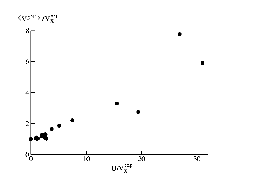
Figure 4: Normalized drift velocity of the chemical front $\langle V_{f}^{exp}\rangle/V_{\chi}^{exp}$ versus the normalized flow intensity $\overline{U}/V_{\chi}^{exp}$.

As mentioned above, it is seen from the instantaneous velocity curve ($V_{f}^{exp}(t)$, figure 3), that the front velocity oscillates at the frequency of the flow. However, due to the experimental noise, it is difficult to obtain further information from this curve.

We also noticed from our observation of the experimental movies that the width of the colored front, $L(t)$, was likely to oscillate at a frequency twice that of the excitation, which, unfortunately, is not obvious on the static pictures (figure 2). We note that this feature could support the description of the front thickness in the framework of an effective diffusion of coefficient $D$, as the latter is expected to be insensitive to the flow direction and to depend only on the flow intensity as $D\propto U^{2}$ [16] (which here oscillates at $2f$).

To test this empirical observation, we measured the width $L(t)$ of the dark blue ribbon. As this ribbon corresponds to the presence of the transient iodine, $L(t)$ is a qualitative measure of the chemical front width, but gives however the right time behavior. A classical Fourier analysis of $L(t)$ was tried, but, due to the large amount of noise, it did not provide any reliable frequency dependence. Therefore, we used the more sensitive micro-Doppler method (see [23, 24] and the references therein) which analyzes an instantaneous signal frequency. The so-obtained oscillation frequencies $f^{\prime}$ of the width $L(t)$ versus the imposed ones $f$, are displayed in figure 5: They collapse onto the straight line $f^{\prime}=2f$, which supports the contention that the front width oscillates at twice the frequency of the flow.

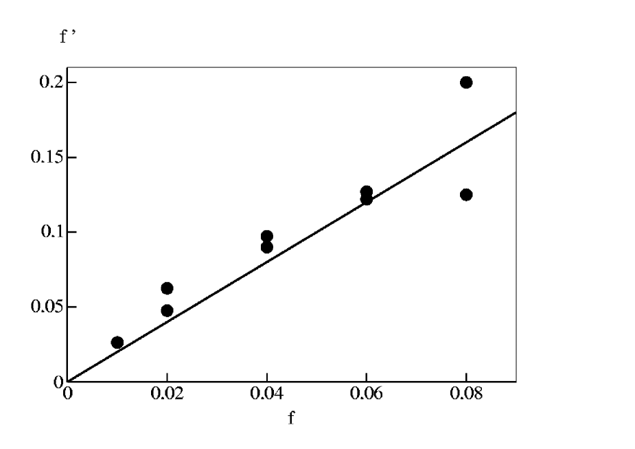
Figure 5: Experimental oscillation frequency $f^{\prime}$ (Hz) of the front width versus the imposed oscillation frequency $f$ of the flow (Hz). $\bullet$: Experimental values obtained with the micro-Doppler algorithm, — : $f^{\prime}=2f$.

In order to have further insight into the instantaneous features of the propagating front, we used numerical simulations, which are less noisy and give access to the behavior in the gap of the cell.

2-D Numerical simulations

Assuming a third-order autocatalytic reaction kinetics for the IAA reaction [1, 6, 13] and a unidirectional flow $U(x,y,t)$ in the $z$ direction, equation (1) reads:

$$\frac{\partial C}{\partial t}+U\frac{\partial C}{\partial z}=D_{m}\left(\frac{\partial^{2}C}{\partial x^{2}}+\frac{\partial^{2}C}{\partial z^{2}}\right)+\alpha C^{2}(1-C)$$ (4)

where $C$ is the concentration of the (autocatalytic) reactant iodide, normalized by the initial concentration of iodate, $D_{m}$ is the molecular diffusion coefficient and $\alpha$ is the kinetic rate coefficient of the reaction. The solution of equation (4) is obtained using a lattice Bhatnagar-Gross-Krook (BGK) method, shown to be efficient in similar contexts [15, 22, 25, 26]. The full $3D$ periodic velocity field $U(x,y,t)$, in a Hele-Shaw cell, has been derived analytically in the Appendix (equation (26)). As mentioned above, the oscillating flow field does not vary much along the $y$ direction (except in a boundary layer of the order of the gap thickness $b$), and the velocity field, away from the side walls, is basically a $2D$ flow field, $U(x,t)$, given by:

$$U(x,t)=U_{M}\Re e\left[\left(1-\frac{\cos{(kx)}}{\cos{(kb/2)}}\right)e^{i\omega t}\right]$$ (5)

where $k=\sqrt{\frac{i\omega}{\nu}}$ is a complex wave number. Note that for small frequency, $\omega\ll\nu/b^{2}$ (i.e. $b\ll l_{\nu}$), equation (5) reduces to an oscillating Poiseuille flow: $U(x,t)\approx U_{M}(1-4x^{2}/b^{2})\sin{(\omega t)}$. The analytic flow field (equation (5)) is used in equation (4) for the $2D$ simulation of the ADR equation by the lattice BGK method.

In order to compare the results of the numerical simulations with the experiments, we used the same non dimensional quantities, namely $b/l_{\chi}^{exp}$ ($=4$), $U_{M}/V_{\chi}^{exp}$ and the Schmidt number $Sc=\nu/D_{m}$ ($=500$) which compares the viscous and mass diffusivities. The simulations were performed on a lattice of length $N_{z}$, ranging between $2000$ and $6000$ nodes, and of constant width $N_{x}=40$ nodes during $2\times 10^{5}$ to $4\times 10^{6}$ iterations. The above experimental value of $b/l_{\chi}^{exp}$ gives a numerical chemical length $l_{\chi}=10=\sqrt{\frac{2D_{m}}{\alpha}}$. We chose $D_{m}=5.10^{-3}$ and $\alpha=10^{-4}$, which sets the front velocity $V_{\chi}=\sqrt{\frac{\alpha D_{m}}{2}}=5.10^{-4}$ and the kinematic viscosity $\nu=D_{m}Sc=2.5$. The varying parameters in the simulations are the amplitude $A$ and the frequency $f$ of the imposed oscillating flow field. A typical movie of a numerical simulation is displayed in figure 6.

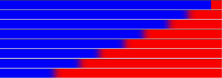
Figure 6: Numerical simulation of the front displacement (obtained with $A=10$ and $f=2.5\times 10^{-6}$). The product of the reaction is in dark and the reactant is in grey. From top to bottom, time increases by $200000$ time steps ($=1/2$ period). The lattice dimensions are $40\times 4000$ (note that the aspect ratio of the pictures is not $1$).

It is seen from these movies that the front oscillates and travels from the burnt product to the fresh reactant. The mean concentration profiles are obtained by averaging along the lattice width, and analyzed along the same line as in the experiments. Figure 7 shows the time evolution of the displacement of the iso-concentration $\overline{C}=0.5$, obtained in the $2D$ simulations and in the experiments: The agreement between the two supports the contention that in our frequency range, the dynamics of the front is governed only by the variations of the velocity field in the gap ($b=0.4\;mm$), and that the (large) transverse extent of the plane of the experimental cells ($h=8\;mm$) plays no role.

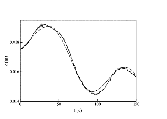
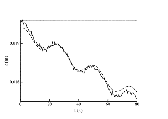
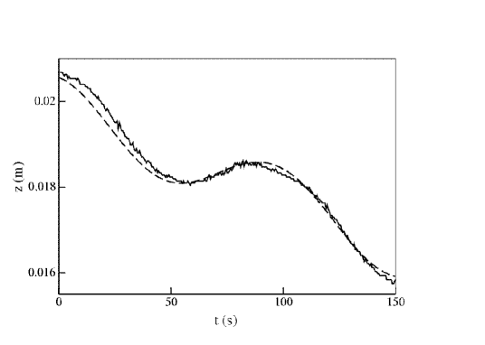
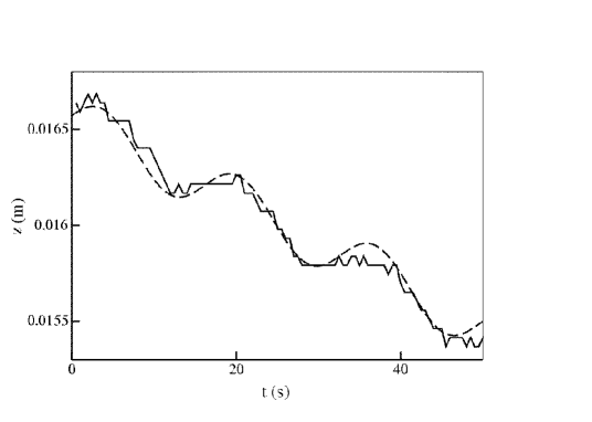
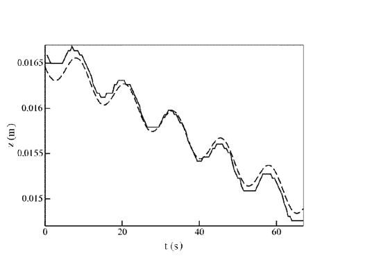
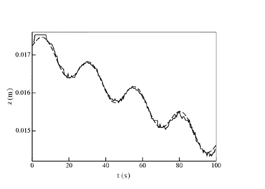
Figure 7: Time evolution of the front position. $-$: Experimental data, $--$: Numerical simulations. The experimental values $(A,f)$ ($A$ in $mm$ and $f$ in $Hz$) are: $(1.12,0.01)$, $(0.55,0.01)$, $(0.14,0.08)$, $(0.27,0.04)$, $(0.1,0.06)$, $(0.14,0.04)$ from top left and clockwise.

Figure 8 displays the resulting normalized drift front velocity $\langle V_{f}\rangle/V_{\chi}$ versus the normalized flow velocity $\overline{U}/V_{\chi}$. The two sets of data, obtained experimentally and numerically, are also in good agreement. This leads us to analyze in more details the dynamics of the front in the gap, with the help of the $2D$ numerical simulations.

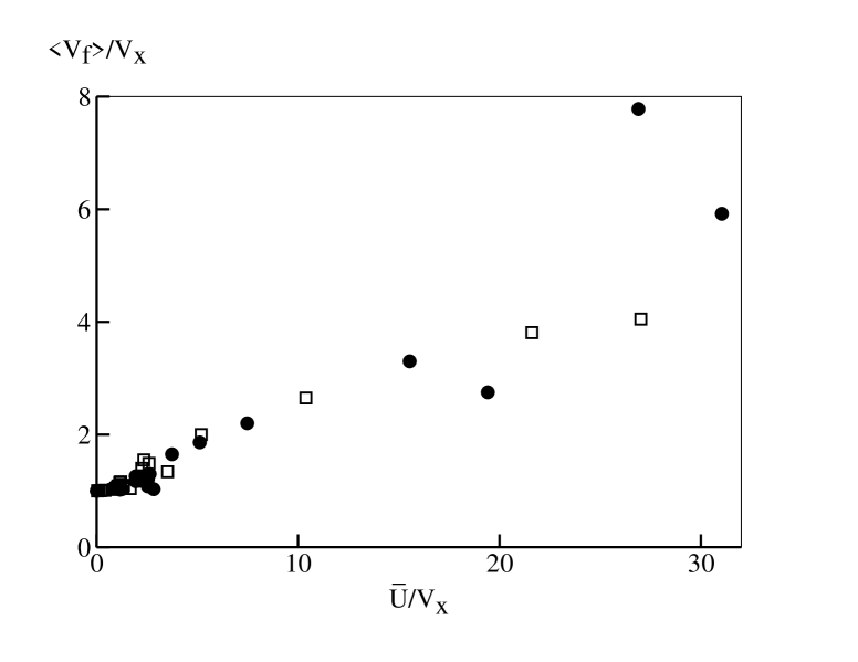
Figure 8: Normalized drift velocity $\langle V_{f}\rangle/V_{\chi}$ versus the normalized flow velocity $\overline{U}/V_{\chi}$. $\bullet$: Experimental data, $\square$: Numerical simulations.

The theoretical front width given in (2) can be obtained from the second-order moment of the derivative of the concentration profile [16]:

$$l_{\chi}^{2}=\frac{3}{\pi^{2}}\int_{-\infty}^{+\infty}z^{2}\frac{d\overline{C}}{dz}dz$$ (6)

The use of the discrete version of (6) allows us to estimate the front width $l_{f}$. Figure 9 displays the time evolution of $l_{f}$.

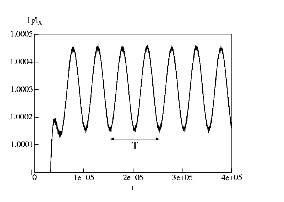
Figure 9: Time evolution of the normalized effective front width $l_{f}/l_{\chi}$ for the numerical simulation $A=10$ and $f=10^{-5}$. The period $T$ of the oscillating flow is indicated for comparison.

After a transient time of the order of one flow period, the front width $l_{f}(t)$ becomes periodic and oscillates with a frequency twice that of the imposed flow, in agreement with the experimental result given in figure 5.

For a stationary laminar flow, we showed in [16] that, under mixing regime conditions, the velocity and width of the reaction front result from a Taylor-like diffusion process, with an effective diffusion coefficient $D_{eff}$ such that $V_{f}=\sqrt{\alpha D_{eff}/2}$ and $l_{f}=\sqrt{2D_{eff}/\alpha}$, leading to $V_{f}/l_{f}=\alpha/2$. An easy way to test the relevance of this effective diffusion description to the present case is to measure the ratio of the time-averaged values $\langle V_{f}\rangle/\langle l_{f}\rangle$. Figure 10 clearly shows that the relation between $\langle V_{f}\rangle$ and $\langle l_{f}\rangle$ is not linear. This allows us to discard the above description.

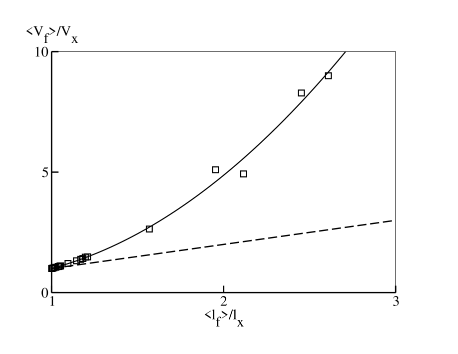
Figure 10: Normalized front velocity $\langle V_{f}\rangle/V_{\chi}$ versus normalized front width $\langle l_{f}\rangle/l_{\chi}$. The line through the data (best quadratic fit) indicates that $\langle V_{f}\rangle/V_{\chi}$ is not proportional to $\langle l_{f}\rangle/l_{\chi}$. Dashed line : $\langle V_{f}\rangle/V_{\chi}=\langle l_{f}\rangle/l_{\chi}$.

The information given by both the experiments and the numerical simulations may be summarized as follows: In the presence of a periodic flow, the propagation of a chemical front in a Hele-Shaw cell is governed by the velocity profile in the gap. The front position drifts in the natural direction of the chemical wave and undergoes oscillations at the frequency of the flow whereas the front width oscillates at twice this frequency. Finally, the front behavior cannot be described in terms of a Taylor-like effective diffusion.

In the next section, we derive a model, under the assumption of weak flow velocity, and discuss the above findings in the light of our theoretical approach.

Theoretical determination of the front velocity

We have derived in a previous work [16], the velocity of a stationary reaction front, using a small parameter expansion method. The two parameters were the reduced gap thickness $b/l_{\chi}$ (or $\eta=b/2l_{\chi}$) and the normalized flow velocity $\varepsilon=\overline{U}/V_{\chi}$, with $\overline{U}=2U_{M}/3$ in $2D$. We shall use the same method in order to derive the instantaneous front velocity and width. We note that this extends the work by Nolen and Xin [12] on the drift front velocity.

The ADR equation in a $2D$, unidirectional flow along $z$ writes:

$$\frac{\partial C}{\partial t}+U\frac{\partial C}{\partial z}=D_{m}\left(\frac{\partial^{2}C}{\partial x^{2}}+\frac{\partial^{2}C}{\partial z^{2}}\right)+\alpha C^{2}(1-C)$$ (7)

The $2D$ flow is imposed in a gap of size extension $b$. We assume a frequency small enough ($l_{\nu}=\sqrt{\nu/\omega}\gg b$) to have an oscillating Poiseuille flow:

$$U(x,t)=U_{M}\left(1-\frac{4x^{2}}{b^{2}}\right)\sin{(\omega t)}$$ (8)

We also assume that the flow velocity is small compared to $V_{\chi}$,

$$\varepsilon=|U_{M}|/V_{\chi}\ll 1$$ (9)

and that, accordingly, the change in the front velocity due to the presence of the flow is small compared to $V_{\chi}$, $(V_{f}(t)-V_{\chi})\ll V_{\chi}$.

Moreover, we assume that the concentration field is nearly uniform along the transverse $x$ direction. Note that, for a passive tracer, this hypothesis is fulfilled when the Péclet number $Pe=|U|b/D_{m}$ is smaller than $L/b$, where $L$ is the typical advection length (condition for Taylor-diffusion regime). In the presence of a reaction, this condition becomes $\varepsilon\eta^{2}\ll 1$ [16]. We recall first the approach of Nolen and Xin [12], in our notations. In the moving frame ($s=z-V_{f}t$), under the assumption (9) of a weak flow velocity ($\varepsilon\ll 1$), the concentration $C(s,x,t)$ and the velocities $U$ and $V_{f}$ can be expanded in powers of $\varepsilon$, as follows:

$$C = C_{0}(s)+\varepsilon C_{1}(s,x,t)$$ (10)

$$U = \varepsilon U_{1}(x,t)$$ (11)

$$V_{f} = V_{\chi}+\varepsilon V_{1}(t)+\varepsilon^{2}V_{2}(t)+...$$ (12)

where $C_{0}(s)=1/(1+e^{s/l_{f}})$ is the mean concentration profile (averaged over the gap and the time) and $C_{1}(s,x,t)$ denotes deviations from the mean. Using the space and time Fourier decomposition of the flow velocity field, $U_{1}=\sum_{n}b_{n}e^{ik_{n}x+i\omega t}$, for a monochromatic ($\omega$) velocity field (where $k_{n}=2n\pi/b$ is the decomposition wave vector for a gap of width $b$), and expanding the ADR equation in the moving frame, Nolen and Xin derived the time-averaged, drift velocity:

$$\langle V_{f}\rangle=V_{\chi}(1+\varepsilon^{2}\gamma/2)\mbox{, with }\gamma=\frac{\eta^{2}}{2\pi^{2}}\sum_{n>0,}\frac{2n^{2}\mid b_{n}\mid^{2}}{\left(n^{4}+\frac{\omega^{2}}{\Omega^{2}}\right)}$$ (13)

where $\Omega=\frac{4\pi^{2}D_{m}}{b^{2}}$ is a characteristic frequency, proportional to the inverse of the typical diffusion time across the gap $b$. For the Poiseuille flow used here, one finds $b_{n}=(-1)^{n}3/\pi^{2}n^{2}$.

In this paper, we are interested in the time dependence of the front velocity, in the presence of a sine flow velocity (a single temporal mode, $\omega$, in the Fourier decomposition of $U_{1}$). After some calculations and with the necessary assumption $\frac{\partial^{2}C_{1}}{\partial x^{2}}\ll\frac{\partial^{2}C_{1}}{\partial s^{2}}$, we find (see [27] for details):

$$\frac{V_{f}}{V_{\chi}}(t)=1+\varepsilon\cos{(\omega t)}+\varepsilon^{2}\eta^{2}[\gamma_{1}(1+\cos{(2\omega t)})+\gamma_{2}\sin{(2\omega t)}]$$ (14)

with

$$\gamma_{1} = \frac{9}{2\pi^{6}}\sum_{n>0}\frac{1}{n^{2}\left(\frac{\omega^{2}}{\Omega^{2}}+n^{4}\right)}$$ (15)

$$\gamma_{2} = \frac{9}{2\pi^{6}}\frac{\omega}{\Omega}\sum_{n>0}\frac{1}{n^{4}\left(\frac{\omega^{2}}{\Omega^{2}}+n^{4}\right)}$$ (16)

The equations (14), (15) and (16) display no term involving $\omega/\alpha$, which demonstrates that the reaction kinetics does not play any role at this order. At first order in $\varepsilon$ the front velocity is the algebraic sum of the gap-averaged flow velocity and of the chemical wave velocity in the absence of flow. Note that this result is surprisingly similar to the one obtained for the front displacement in constant flows in the mixing regime [14, 16]. The leading order pulsative flow contribution causes the front to oscillate with the flow frequency. At second order in $\varepsilon$, the contributions to the front velocity are a constant one and one at twice the frequency of the flow field. Note that for $\omega=0$, we recover previous results: $\frac{V_{f}}{V_{\chi}}\approx 1+\varepsilon+\frac{1}{105}\varepsilon^{2}\eta^{2}$ [9, 14, 16]. Averaging expression (14) over one period leads to the drift front velocity (13) $\langle V_{f}^{theo}\rangle/V_{\chi}=1+\varepsilon^{2}\eta^{2}\gamma_{1}$. We note that the amplitude $K_{v}$ of the velocity oscillation is mainly dominated by the order one term: $K_{v}\simeq\varepsilon$. Figure 11 shows that the theoretical results and the numerical simulation data for the drift velocity and its amplitude of oscillation are in reasonable agreement for small $\varepsilon$ ($\varepsilon<1$).

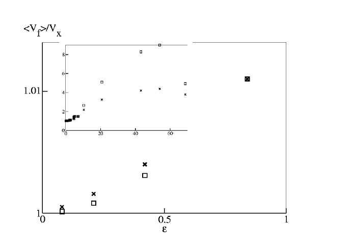
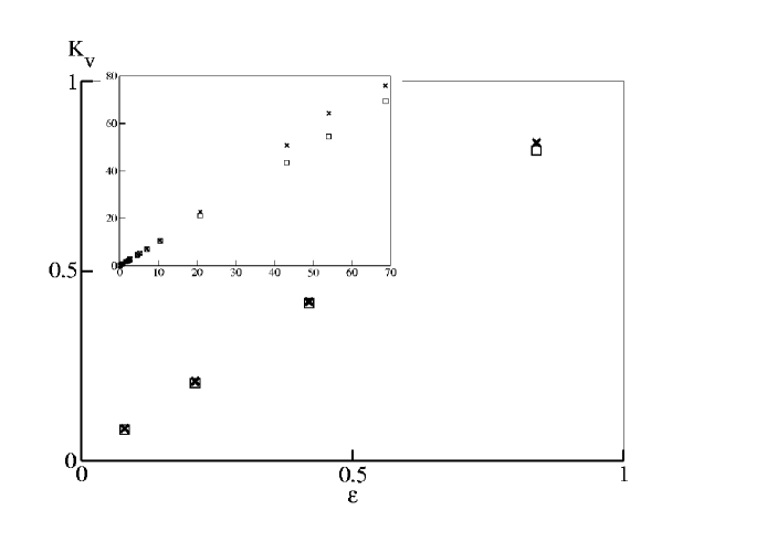
Figure 11: Left: Normalized drift front velocity $\langle V_{f}\rangle/V_{\chi}$ versus $\varepsilon=|U_{M}|/V_{\chi}$. $\square$: Numerical simulation data, $X$: Theoretical predictions in the limit of small $\varepsilon$.
Right: Amplitude $K_{v}$ of the oscillation of $V_{f}(t)/V_{\chi}$ versus $\varepsilon$. $\square$: Simulations results, $X$: Theoretical results.
The insets give the behavior of $\langle V_{f}\rangle/V_{\chi}$ and $K_{v}$ over a wider range of $\varepsilon$.

Conclusion

In this paper, we have analyzed the influence of a time-periodic flow on the behavior of an autocatalytic reaction front. The numerical simulations are in reasonable agreement with the experiments and show that the front dynamics is controlled by the flow velocity in the gap of a Hele-Shaw cell in the range of the parameters explored. We have shown that, contrary to the case of a stationary laminar flow, a Taylor-like approach cannot account for the (time-averaged) width and velocity of the front. The instantaneous front velocity has been derived theoretically, in the weak flow velocity regime. It is found to be in reasonable agreement with the numerical simulation results for $|U_{M}|/V_{\chi}<1$.

Appendix : Determination of the oscillating velocity profile in a Hele-Shaw cell

We consider a laminar flow, unidirectional along the $z$ direction, in a Hele-Shaw cell of cross-section $b\times h$ ($b\ll h$) in the $x$ and $y$ directions, respectively. The Navier-Stokes equation in the $z$ direction writes:

$$\frac{\partial U}{\partial t}=\nu\left(\frac{\partial^{2}U}{\partial x^{2}}+\frac{\partial^{2}U}{\partial y^{2}}\right)-\frac{1}{\rho}\frac{\partial P}{\partial z}e^{-i\omega t}$$ (17)

where a harmonic pressure gradient oscillating at frequency $f=\omega/2\pi$ is imposed, and the flow velocity $U(x,y,t)$ satisfies the boundary conditions:

$$U(x,\pm\frac{h}{2},t)=U(\pm\frac{b}{2},y,t)=0$$ (18)

In order to derive the analytical expression of $U$, we extend the method used by Gondret et al [22] to calculate the stationary flow field. First, we consider the flow field, written $U^{*}(x)e^{-i\omega t}$, between two infinite planes (at $x=\pm\frac{b}{2}$ as in our simulations), which satisfies:

$$\frac{\partial^{2}U^{*}}{\partial x^{2}}+\frac{i\omega}{\nu}U^{*}=\frac{1}{\rho\nu}\frac{\partial P}{\partial z}$$ (19)

leading to [21]:

$$U^{*}(x)=\frac{1}{i\omega\rho}\frac{\partial P}{\partial z}\left[1-\frac{\cos{(kx)}}{\cos{\left(\frac{kb}{2}\right)}}\right]$$ (20)

where $k=\sqrt{\frac{i\omega}{\nu}}=(1+i)\sqrt{\frac{\omega}{2\nu}}$. Following [22], we write now the solution of the full problem as:

$$U(x,y,t)=\left[U^{*}(x)+U^{**}(x,y)\right]e^{-i\omega t}$$ (21)

where $U^{**}(x,y)$ must now satisfy:

$$\frac{\partial^{2}U^{**}}{\partial x^{2}}+\frac{\partial^{2}U^{**}}{\partial y^{2}}+\frac{i\omega}{\nu}U^{**}=0$$ (22)

with the boundary conditions:

$$U^{**}(\pm\frac{b}{2},y) = 0$$ (23)

$$U^{**}(x,\pm\frac{h}{2}) = -U^{*}(x)$$ (24)

The solution of (22) is found assuming a Fourier decomposition of the form:

$$U^{**}(x,y)=\sum_{n=1}^{\infty}A_{n}\cos{(k_{xn}x)}\cos{(k_{yn}y)}$$ (25)

where $k_{xn}=(2n-1)\pi/b$, in order to satisfy the boundary condition (24). After some calculations, we obtain the solution of (17):

$$U(x,y,t)=-\frac{ie^{-i\omega t}}{\omega\rho}\frac{\partial P}{\partial z}\left[1-\frac{\cos{(kx)}}{\cos{\left(\frac{kb}{2}\right)}}+\sum_{n=1}^{\infty}4(-1)^{n}\frac{k^{2}\cos{(k_{xn}x)}\cos{(k_{yn}y)}}{(2n-1)\pi k_{yn}^{2}\cos{\left(k_{yn}\frac{h}{2}\right)}}\right]$$ (26)

where $k_{yn}^{2}=\frac{i\omega}{\nu}-k_{xn}^{2}$. The velocity $U(x,y,t)$ induced by an oscillating pressure gradient has a phase shift and a modulus which depend on space. We note that the maximum modulus $U_{M}$ occurs in the middle of the cell ($x=y=0$). In Expression (26), the first two terms correspond to a 2D oscillating flow between two parallel boundaries at distance $b$ ($U^{*}$) [21], and the third one accounts for the finite size of the cell in the larger direction $h$ ($U^{**}$). We note that at high frequency, a plug flow takes place in the section of the cell, except in a thin viscous layer $l_{\nu}=\sqrt{\nu/\omega}$ close to the boundaries ($y=\pm h/2$ and $x=\pm b/2$). On the opposite, in the low frequency regime ($l_{\nu}\gg b$), the oscillating flow has the same shape as a static one given in [22]. Hence, except in a thin layer (of thickness $\sim b\ll h$) close to the side boundaries ($y=\pm h/2$), the flow is a parabolic Poiseuille flow of the form:

$$U(x,t)=U_{M}\left(1-\frac{4x^{2}}{b^{2}}\right)\sin{(\omega t)}$$ (27)

References

- [1] S. K. Scott, Oxford University Press, Oxford (GB) (1994).
- [2] P. Clavin, Prog. Energy. Combust. Sci. 11, 1 (1985).
- [3] R. A. Fisher, Pro. Annu. Symp. Eugenics. Soc. 7, 355 (1937).
- [4] A. N. Kolmogorov, I. G. Petrovskii and N. S. Piskunov, Moscow Univ. Math. Bull. (Engl. Transl.) 1, 1 (1937).
- [5] P. A. Epik and N. S. Shub, Dokl. Akad. Nauk SSSR 100, 503 (1955).
- [6] A. Hanna, A. Saul and K. Showalter, J. Am. Chem. Soc 104, 3838 (1982).
- [7] Ya. B. Zeldovitch and D. A. Franck-Kamenetskii, Actu. Phys. USSR. 9, 341 (1938).
- [8] U. Ebert and W. van Saarloos, Physica D 146, 1 (2000).
- [9] G. Papanicolaou and J. Xin, J. Stat. Phys. 63, 915 (1991).
- [10] B. Audoly, H. Berestycki and Y. Pomeau, C. R. Acad. Sc. Paris, Series IIb 328, 255 (2000).
- [11] M. Abel, A. Celani, D. Vergni and A. Vulpiani, Phys. Rev. E. 64, 046307 (2001).
- [12] J. Nolen and J. Xin, SIAM J. Multiscale Modeling and Simulation 1, 554 (2003).
- [13] M. Böckmann and S. C. Müller, Phys. Rev. Lett. 85, 2506 (2000).
- [14] B. F. Edwards, Phys. Rev. Lett. 89, 104501 (2002).
- [15] M. Leconte J. Martin, N. Rakotomalala and D. Salin, Phys. Rev Lett 90, 128302 (2003).
- [16] M. Leconte J. Martin, N. Rakotomalala, D. Salin and Y. C. Yortsos, J. Chem. Phys. 120, 7314 (2004).
- [17] G.I. Taylor, Proc. Roy. Soc. Lond. A 219, 186 (1953). G. I. Taylor, Proc. Roy. Soc. B 67, 857 (1954).
- [18] P. C. Chatwin, J. Fluid. Mech. 71, 513 (1975).
- [19] R. Smith, J. Fluid. Mech. 114, 379 (1982).
- [20] E. J. Watson, J. Fluid. Mech. 133, 233 (1983).
- [21] L. Landau and E. Lifchitz, ”Physique théorique, mécanique des fluides” Mir edition, (1989).
- [22] P. Gondret, N. Rakotomalala, M. Rabaud, D. Salin and P. Watzky, Phys. Fluids. 9, 1841 (1997).
- [23] I. Renhorn, C. Karlsson, D. Letalick, M. Millnert and R. Rutgers, SPIE 2472, 23 (1995).
- [24] M. Lavielle and C. Lévy-Leduc, to appear in IEEE Transaction On Signal Processing, (2005).
- [25] J. Martin, N. Rakotomalala, D. Salin and M. Böckmann, Phys. Rev E, 65 051605 (2002).
- [26] N. Rakotomalala, D. Salin and P. Watzky, J. Fluid. Mech. 338, 277 (1997).
- [27] M. Leconte, ”Propagation de front de réaction sous écoulement”, Thèse de doctorat, (2004).