Design of switches and beam splitters using chaotic cavities

O. Bendix and J. A. Méndez-Bermúdez

Max-Planck-Institut für Dynamik und Selbstorganisation, Bunsenstraße 10, D-37073 Göttingen, Germany

Abstract

We propose the construction of electromagnetic (or electronic) switches and beam splitters using chaotic two-dimensional multi-port waveguides. A prototype two-port waveguide is locally deformed in order to produce a ternary incomplete horseshoe proper of mixed phase space (chaotic regions surrounding islands of stability where motion is regular). Due to tunneling to the phase space stability islands the appearance of quasi-bound states (QBS) is induced. Then, we attach transversal ports to the waveguide on the deformation region in positions where the phase space structure is only slightly perturbed. We show how QBS can be guided out of the waveguide through the attached transversal ports giving rise to frequency selective switches and beam splitters.

OCIS codes:  230.1360, 230.7370, 270.3100.

Switches and beam splitters are key elements in optical information processing, imaging, integrated photonic, and optical communication systems. In this letter we propose a novel way to construct switches and beam splitters using two-dimensional (2D) chaotic waveguides.

The 2D waveguide we shall use is formed by a cavity connected to two collinear semi-infinite ports of width $d$ extended along the $x$-axis. The prototype cavity has the geometry of the so-called cosine billiard[1, 2, 3, 4]: it has a flat wall at $y=0$ and a deformed wall given by $y(x)=d+a[1-\cos(2\pi x/L)]$, where $a$ is the amplitude of the deformation and $L$ is the length of the cavity. In Fig. 1(a) we show the geometry of the waveguide.

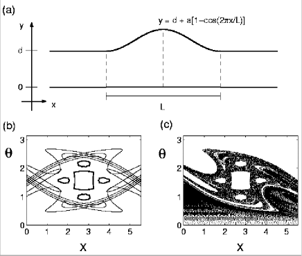
Fig. 1: (a) Geometry of the waveguide, (b) horseshoe, and (c) transient Poincarè map with surface of section at $y=0$, $(d,a,L)=(1.0,0.305,5.55)$. The tendrils[5] of the horseshoe in (b) are plotted up to level three. The thick lines in (b) are the limits of stability islands. The transient Poincarè maps in (c) is constructed for rays entering the cavity from the left port.

In order to obtain the panorama of the ray (classical) dynamics of the waveguide we construct its Smale horseshoe[5]. It gives the topology of the homoclinic tangle which completely characterizes the scattering dynamics, connecting the interacting region with the asymptotic regions. For our waveguide, the domain of the interacting region is the cavity, while the asymptotic regions are the ports. The number of fundamental orbits (period-one periodic orbits) determine the order of the horseshoe. Our cavity (for $a>0$) has three of them (shown in dashed lines in Fig. 1(a)) and hence its horseshoe is ternary. The horseshoe is formed by the invariant manifolds (stable and unstable) of the hyperbolic fixed points of the cavity (the ones located at the edges of the cavity). We plot the horseshoe using a Poincarè Map[6] (PM), i.e., we follow orbits with initial conditions along the manifolds and each time a ray impinges on the flat wall of the waveguide (chosen as surface of section) we plot the position $x$ and the angle $\theta$, the angle the ray makes with the lower boundary. In Fig. 1(b) we present the horseshoe of the waveguide with parameters $(d,a,L)=(1.0,0.305,5.55)$ where only the tendrils[5] up to the hierarchy level three are plotted. In particular for this set of parameters the horseshoe is incomplete; a typical situation of mixed phase space.

For the set of parameters used here, the cavity develops a period-one and period-four resonance islands whose boundaries are shown with thick lines in Fig. 1(b). These islands are formed by trapped orbits bouncing in the neighborhood of stable periodic orbits. In particular the central island is formed by trajectories colliding nearly perpendicular with the walls around $x=L/2$. Note that the orbits within these islands are not accessible to scattering rays.

To further analyze our waveguide system we use the transient Poincarè map[3] which is a PM where the initial conditions are chosen to lie outside the cavity. The transient PM generated by trajectories whose initial conditions start in the left port is presented in Fig. 1(c). Comparison of Fig. 1(b) and Fig. 1(c) shows, as expected, that the stability islands produced by bounded motion inside the cavity are forbidden phase space regions for scattering trajectories. Also note that the structure of the transient PM shadows the unstable manifold of the corresponding horseshoe.

To study the wave scattering phenomena we numerically solve the Schrödinger equation to compute the scattering wave functions (by means of the Fisher-Lee relation[7]) and the energy-dependent conductance $G_{pq}$ (using the Landauer-Büttiker formalism[7]), measured from port $q$ to port $p$. We want to emphasize that since the problem of a quantum wave in a 2D billiard (Schrödinger equation) is equivalent to that of a TM wave inside a 2D waveguide with Dirichlet boundary conditions (Helmholtz equation)[8], our analysis is applicable to both, electronic and electromagnetic setups.

Additionally, to explore ray-wave correspondence we use the Husimi distribution[9] which is the projection of a given state onto a coherent state of minimum uncertainty. The Husimi distribution is a phase space probability density that can be directly compared to the ray phase space.

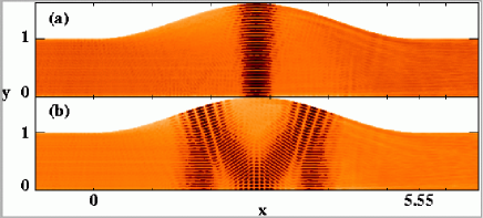
Fig. 2: Density plots for scattering wave functions calculated at resonance energies (light-dark = minimum-maximum). (a) $E=4008.8583$, (b) $E=4027.0597$. These QBS are constructed by averaging all the ${\cal M}=20$ open modes. $E=2d^{2}E_{\mbox{\tiny W}}\sim{\cal M}^{2}\pi^{2}$; where $E_{\mbox{\tiny W}}$ is the energy of the wave and ${\cal M}$ is the largest transversal mode $m$ beyond which the longitudinal wave vector $[2E_{\mbox{\tiny W}}-(m\pi/d)^{2}]^{1/2}$ becomes complex.

It has been shown[3, 4] that when the cavity of the waveguide of Fig. 1(a) is characterized by an incomplete horseshoe the conductance $G_{\mbox{\tiny LR}}$ (= $G_{\mbox{\tiny RL}}$) fluctuates strongly with sharp resonances. The wave functions belonging to the sharpest conductance resonances can be identified with energy eigenstates living in the phase space stability islands. In particular, we noticed[10] that some wave functions at resonance reveal I-, V- and M-shaped patterns which shadow the ray trajectory of a particle in a period one, two and four periodic orbits, respectively. The reason of this phenomenon is Heisenberg’s uncertainty principle that allows scattering wave functions to tunnel through KAM barriers[6]. Since the scattering wave functions that tunnel into classical islands are very similar to a set of eigenfunctions of the corresponding closed cavity, we named them quasi bound states (QBS). For the set of parameters chosen for the cavity in this work, the QBS may be of two types only: I-type or M-type. See the corresponding scattering wave functions in Fig. 2 found at $G_{\mbox{\tiny LR}}$ local minima for waves incident from the left port. Notice that under resonance conditions the cavity acts as a resonator. The I-type (M-type) QBS have support on the period-one (period-four) resonance island, as can be clearly seen in Fig. 5(a-b) where we plot the Husimi distributions for the QBS of Fig. 2 together with the transient PM of the system.

Now, the idea is to attach transversal ports to the cavity in order to guide the QBS out of the waveguide (once they are excited by the appropriate resonance energy) to construct switches and/or beam splitters. Without loss of generality, we will attach semi-infinite ports of width $d_{\mbox{\tiny T}}$ extended along the $y$-axis (see some multi-port setups in Fig. 3). Then, to make use of the I-type QBS the ports have to be attached to the waveguide centered at $x=L/2$ (the position of the period-one periodic orbit supporting I-type QBS) on the lower boundary, on the upper one [Fig. 3(a)], or on both [Fig. 3(d)]. While to use the M-type QBS, the ports should be centered at $x=L/2$ and $L/2\pm 0.975$ on the lower boundary or/and at $x=L/2\pm 0.975$ on the upper one, see for example Figs. 3(b,e,f). In particular we will use the setup of Fig. 3(c) which combines both, I- and M-type QBS.

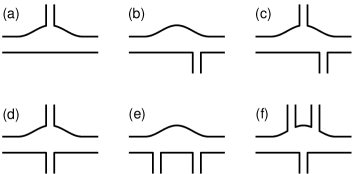
Fig. 3: Examples of (a-c) switch and (d-f) beam splitter setups.

Evidently, by attaching transversal ports to the waveguide the cavity phase space is perturbed. However since we want to make use of QBS, the width $d_{\mbox{\tiny T}}$ of the attached ports must be small enough to preserve the global phase space structure. Then, in Fig. 4 we analyze the effect of the size of the transversal ports on the phase space for the setup of Fig. 3(c) by plotting the transient PM for different values of $d_{\mbox{\tiny T}}$. Notice that by increasing $d_{\mbox{\tiny T}}$, the chaotic region separating the period-one and period-four stability islands becomes narrower until it completely disappears. Thus, we will use a value of $d_{\mbox{\tiny T}}$ for which the transient PM still shows period-one and period-four stability regions: $d_{\mbox{\tiny T}}=0.15$, see Fig. 4(c).

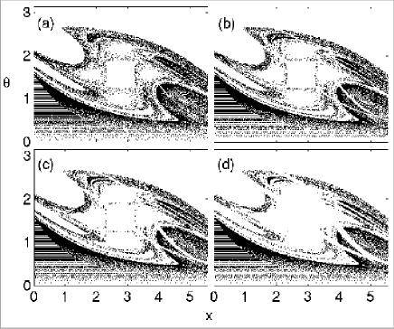
Fig. 4: Transient Poincarè maps with surface of section at $y=0$ constructed for rays entering the beam splitter setup of Fig. 3(c) from the left port. (a) $d_{\mbox{\tiny T}}=0.05$, (b) $d_{\mbox{\tiny T}}=0.10$, (c) $d_{\mbox{\tiny T}}=0.15$, and (d) $d_{\mbox{\tiny T}}=0.25$.

Remember that the QBS shown in Fig. 2 are produced at frequencies that correspond to sharp local minima in $G_{\mbox{\tiny LR}}$. Now, for the multi-port setup of Fig. 3(c) we can also measure the conductance from the left to the upper port, $G_{\mbox{\tiny LU}}$, and from the left to the lower port, $G_{\mbox{\tiny LD}}$. We observe, as expected, that some of the sharpest minima in $G_{\mbox{\tiny LR}}$ correspond to maxima in $G_{\mbox{\tiny LU}}$ or $G_{\mbox{\tiny LD}}$, meaning that at such frequencies a wave tunneling to the stability regions is guided up or down through the transversal ports. To show such behavior, in Fig. 5 we compare the Husimi distributions for the QBS of Fig. 2 (waveguide without transversal ports) to Husimi distributions for scattering states at $G_{\mbox{\tiny LR}}$ resonance for the muti-port setup Fig. 3(c). The states of Figs. 5(c) and 5(d) correspond to minima in $G_{\mbox{\tiny LR}}$ and maxima in $G_{\mbox{\tiny LU}}$ and $G_{\mbox{\tiny LD}}$, respectively. As expected since $G_{\mbox{\tiny LR}}$ is minimum, the maximum probability of the Husimi distributions for these states is located inside phase space stability regions (as the QBS of the two-port terminal do). However, there is a probability minimum (equal to zero) at the center of the stable regions indicating that in fact the QBS are guided out from the cavity through the transversal ports.

Note that with the setup of Fig. 3(c) one is able to guide a beam up (down) by exciting an I- (M-) type QBS, thus, giving rise to a frequency selective switch. While, a beam splitter may be constructed by using the setup of Fig. 3(d) (Fig. 3(e)), since an I- (M-) type QBS could be splitted up and down (down) at certain resonant frequencies. Moreover, by the appropriate choice of the geometrical parameters of the cavity one can excite different types of QBS (V-, W-, $\Pi$-type, for example), allowing in this way diverse device designing.

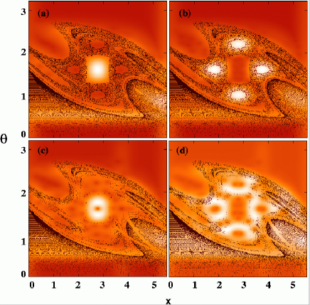
Fig. 5: Transient Poincarè maps (dots) and Husimi distributions (orange-white = minimum-maximum) with surface of section at $y=0$ constructed for rays/waves entering the waveguide of (a-b) Fig. 1(a) and (c-d) Fig. 3(c) from the left port. In (a) and (b) the Husimi distributions for the QBS of Fig. 2(a) and Fig. 2(b) are shown, respectively. In (c) and (d) the Husimi distributions for scattering sates at $G_{\mbox{\tiny LU}}$ and $G_{\mbox{\tiny LD}}$ maxima are plotted, respectively, both at $G_{\mbox{\tiny LR}}$ minima. (c) $E=3997.34$, (d) $E=4103.4096$.

In summary, we have proposed the construction of frequency selective switches and beam splitters using 2D multi-port waveguides. Using ray as well as wave dynamics we shown that the switching and splitting mechanism is based on tunneling into classically forbidden phase space regions. Finally, we want to stress that the choice of the cosine billiard as waveguide cavity does not restrict the applicability of our results, since the construction of frequency selective switches and beam splitters, as described above, only requires a cavity characterized by an incomplete horseshoe.

JAMB (antonio@chaos.gwdg.de) thanks support from the GIF, the German-Israeli Foundation for Scientific Research and Development. We thank J. P. Bird, R. Fleischmann and G. A. Luna-Acosta for useful discussions.

References

- [1] G.B. Akguc and L.E. Reichl, Phys. Rev. E 67, 046202 (2003).
- [2] J.A. Méndez-Bermúdez, G.A. Luna-Acosta, and F.M. Izrailev, Physica E 22, 881 (2004).
- [3] J.A. Méndez-Bermúdez, G.A. Luna-Acosta, P. Šeba, and K.N. Pichugin, Phys. Rev. E 66, 046207 (2002).
- [4] A. Bäcker, A. Manze, B. Huckestein, and R. Ketzmerick, Phys. Rev. E 66, 016211 (2002).
- [5] J. Guckenheimer and P. Holmes, Nonlinear Oscillations, Dynamical Systems, and Bifurcations of Vector Fields (Springer-Verlag, NY, 1983).
- [6] A.J. Lichtenberg and M.A. Lieberman, Regular and Chaotic Dynamics, 2nd Edition (Springer-Verlag, NY, 1992).
- [7] S. Datta, Electronic Transport in Mesoscopic Systems (Cambridge University Press, Cambrige, 1995).
- [8] H.-J. Stöckmann, Quantum chaos: an introduction (Cambridge University Press, Cambrige, 1999).
- [9] K. Husimi, Proc. Phys. Math. Soc. (Jpn.) 22, 246 (1940).
- [10] J.A. Méndez-Bermúdez, G.A. Luna-Acosta, P. Šeba, and K.N. Pichugin, Phys. Rev. B 67, 161104(R) (2003).