Power laws and self-similar behavior in negative ionization fronts

Abstract

We study anode-directed ionization fronts in curved geometries. When the magnetic effects can be neglected, an electric shielding factor determines the behavior of the electric field and the charged particle densities. From a minimal streamer model, a Burgers type equation which governs the dynamics of the electric shielding factor is obtained. A Lagrangian formulation is then derived to analyze the ionization fronts. Power laws for the velocity and the amplitude of streamer fronts are observed numerically and calculated analytically by using the shielding factor formulation. The phenomenon of geometrical diffusion is explained and clarified, and a universal self-similar asymptotic behavior is derived.

I Introduction

In a perfect dielectric medium, charged particles form electrically neutral atoms and molecules due to powerful electric forces. Since there are not free charges in this medium, electric current does not flow inside it. However, if a very strong electric field is applied to a medium of low conductivity in such a way that some electrons or ions are created, then mobile charges can generate an avalanche of more charges by impact ionization, so that a low temperature plasma is created, and an electric discharge develops Rai . This process is called electric breakdown and it is a threshold process: there are not changes in the state of the medium while the electric field across a discharge gap is gradually increased, but at a certain value of the field a current is created and observed.

A streamer is a ionization wave propagating inside a non-ionized medium, that leaves a non-equilibrium plasma behind it. They appear in nature and in technology Rai ; Eddie . A streamer discharge can be modelled using a fluid approximation based on kinetic theory guo . Defining the electron density $N_{e}$ as the integral of the electron distribution function over all possible velocities, we get

$$\frac{\partial N_{e}}{\partial\tau}+\nabla_{\bf R}\cdot{\bf J}_{e}=S_{e},$$ (1)

where $\tau$ is the physical time, $\nabla_{\bf R}$ is the gradient in configuration space, ${\bf U}_{e}({\bf R},\tau)$ is the average (fluid) velocity of electrons, $S_{e}$ is the source term, i.e. the net creation rate of electrons per unit volume as a result of collisions, and ${\bf J}_{e}({\bf R},\tau)=N_{e}({\bf R},\tau)\,{\bf U}_{e}({\bf R},\tau)$ is the electron current density. Similar expressions can be obtained for positive $N_{p}$ and negative $N_{n}$ ion densities.

A usual procedure is to approximate the electron current ${\bf J}_{e}$ as the sum of a drift (electric force) and a diffusion term

$${\bf J}_{e}=-\mu_{e}{\boldsymbol{\cal E}}N_{e}-D_{e}\nabla_{\bf R}N_{e},$$ (2)

where ${\boldsymbol{\cal E}}$ is the total electric field (the sum of the external electric field applied to initiate the propagation of a ionization wave and the electric field created by the local point charges) and $\mu_{e}$ and $D_{e}$ are the mobility and diffusion coefficients of the electrons. Note that, as the initial charge density is low and there is no applied magnetic field, the magnetic effects in equation (2) are neglected. This could not be done in cases where the medium is almost completely ionized or cases in which an external magnetic field is applied, leading to different treatments Chandra .

Some physical processes can be considered giving rise to the source terms. The most important of them are impact ionization (an accelerated electron collides with a neutral molecule and ionizes it), attachment (an electron may become attached when collides with a neutral gas atom or molecule, forming a negative ion), recombination (a free electron with a positive ion or a negative ion with a positive ion) and photoionization (the photons created by recombination or scattering processes can interact with a neutral atom or molecule, producing a free electron and a positive ion) liu .

It is also necessary to impose equations for the evolution of the electric field ${\boldsymbol{\cal E}}$. It is usual to consider that this evolution is given by Poisson’s law,

$$\nabla_{\bf R}\cdot{\boldsymbol{\cal E}}=\frac{e}{\varepsilon_{0}}\,\left(N_{p}-N_{n}-N_{e}\right),$$ (3)

where $e$ is the absolute value of the electron charge, $\varepsilon_{0}$ is the permittivity of the gas, and we are assuming that the absolute value of the charge of positive and negative ions is $e$.

Some simplifications can be made when the streamer development out of a macroscopic initial ionization seed is considered in a non-attaching gas like argon or nitrogen. For such gases, attachment, recombination and photoionization processes are usually neglected. A minimal model turns out and has been used to study the basics of streamer dynamics DW ; Vit ; Ute ; ME ; ME1 ; Andrea . In those cases the evolution of electron and positive ion densities in early stages of the discharge can be written as

$$\frac{\partial N_{e}}{\partial\tau} = \nabla_{\bf R}\cdot\left(\mu_{e}{\boldsymbol{\cal E}}N_{e}+D_{e}\nabla_{\bf R}N_{e}\right)+\nu_{i}N_{e},$$ (4)

$$\frac{\partial N_{p}}{\partial\tau} = \nu_{i}N_{e}.$$ (5)

On time scales of interest the ion current is more than two orders of magnitude smaller than the electron one so it is neglected in (5). In these equations $\nu_{i}N_{e}$ is a term accounting for impact ionization, in which the ionization coefficient $\nu_{i}$ is given by the phenomenological Townsend’s approximation,

$$\nu_{i}=\mu_{e}|{\boldsymbol{\cal E}}|\alpha_{0}e^{-{\cal E}_{0}/|{\boldsymbol{\cal E}}|},$$ (6)

where $\mu_{e}$ is the electron mobility, $\alpha_{0}$ is the inverse of ionization length, and ${\cal E}_{0}$ is the characteristic impact ionization electric field.

It is convenient to reduce the equations to dimensionless form. The natural units are given by the ionization length $R_{0}=\alpha_{0}^{-1}$, the characteristic impact ionization field ${\cal E}_{0}$, and the electron mobility $\mu_{e}$, which lead to the velocity scale $U_{0}=\mu_{e}{\cal E}_{0}$, and the time scale $\tau_{0}=R_{0}/U_{0}$. The values for these quantities for nitrogen at normal conditions are $\alpha_{0}^{-1}\approx 2.3\,\mu\mathrm{m}$, ${\cal E}_{0}\approx 200$  kV/m, and $\mu_{e}\approx 380\,\mathrm{cm^{2}/(Vs)}$. We introduce the dimensionless variables ${\bf r}={\bf R}/R_{0}$, $t=\tau/\tau_{0}$, the dimensionless field ${\bf E}={\boldsymbol{\cal E}}/{\cal E}_{0}$, the dimensionless electron and positive ion particle densities $n_{e}=N_{e}/N_{0}$ and $n_{p}=N_{p}/N_{0}$ with $N_{0}=\varepsilon_{0}{\cal E}_{0}/(eR_{0})$, and the dimensionless diffusion constant $D=D_{e}/(R_{0}U_{0})$.

In terms of the dimensionless variables, the minimal model equations become

$$\frac{\partial n_{e}}{\partial t} = \nabla\cdot{\bf j}+n_{e}f(|{\bf E}|),$$ (7)

$$\frac{\partial n_{p}}{\partial t} = n_{e}f(|{\bf E}|),$$ (8)

$$n_{p}-n_{e} = \nabla\cdot{\bf E},$$ (9)

$${\bf j} = n_{e}{\bf E}+D\;\nabla n_{e},$$ (10)

$$f(|{\bf E}|) = |{\bf E}|e^{-1/|{\bf E}|},$$ (11)

where $\nabla=\nabla_{\bf r}$, and ${\bf j}$ is the dimensionless electron current density.

Some properties of planar fronts have been obtained analytically Ute ; pulled1 ; AJP for the minimal model. A spontaneous branching of the streamers from numerical simulations has been observed ME , as it occurs in experimental situations Pasko . In order to understand this branching, the dispersion relation for transversal Fourier-modes of planar negative shock fronts (without diffusion) has been derived ME1 . For perturbations of small wave number $k$, the planar shock front becomes unstable with a linear growth rate $|E_{\infty}|k$. It has been also shown that all the modes with large enough wave number $k$ (small wave length perturbations) grow at the same rate (it does not depend on $k$ when $k$ is large). However, it could be expected from the physics of the problem that a particular mode would be selected. To address this problem, a possibility is to consider the effect of diffusion. It is also interesting to investigate the effect of electric screening since, in the case of curved geometries, this screening might be sufficient to select one particular mode.

In this paper, we study the properties and structure of anode-directed ionization fronts with zero diffusion coefficient for curved geometries. We start discussing the consequences of neglecting the magnetic field effects in the physics of the streamer evolution. As a consequence, an electric shielding factor can be introduced which determines the behavior of the electric field and the particle densities. From the minimal streamer model, a Burgers type equation which govern the dynamics of the electric shielding factor is deduced. This allows us to consider a Lagrangian formulation of the problem simplifying the analytical and numerical study of the fronts. We apply this new formulation to planar as well as curved geometries (typical in experimental set-ups). Power laws for the velocity and the amplitude of streamer fronts are observed numerically. Theses laws are also calculated analytically by using the shielding factor formulation. The geometrical diffusion phenomenon presented in aft is explained and clarified, and a universal self-similar asymptotic behavior is derived.

The organization of the paper is as follows. In Section II, we will show that all the physics involved in the minimal model can be rewritten in terms of the electric shielding factor, that determines the behavior of the charge densities and the local electric field in the medium. This allows a simple analysis of the model when written in Lagrangian coordinates. Within this framework, we perform in Section III, as an illustration of the Lagrangian formulation, the analysis of planar fronts (without diffusion). In Section IV, we study the evolution of ionization fronts in which the initial seed of ionization is such that the electron density vanishes strictly beyond a certain point for cylindrical and spherical symmetries. We obtain precise power laws for both the velocity of the moving fronts and their amplitude. In Section V, we analyze the special features that appear if the initial seed of ionization is not completely localized but the charge densities slowly decrease along the direction of propagation. For curved geometries, this initial distribution gives rise to a new diffusion-type behavior that we call geometrical diffusion. A universal self-similar asymptotic shape of the fronts is predicted and observed. In Section VI, we establish our conclusions.

II Electric shielding factor

In this section we will reformulate the problem of the evolution of streamer fronts in the minimal model by introducing a new quantity called the electric shielding factor, as in aft . The equation describing the evolution of the shielding factor makes easier the study of curved ionization fronts.

We begin with a brief discussion about the consequences of neglecting the magnetic effects in the minimal streamer model. In this model, it is assumed that the magnetic field effects are negligible, in a first approximation, because (i) the fluid velocity of the electrons is much smaller than the velocity of light, and (ii) the initial magnetic field is zero. Strictly speaking, if the magnetic field is zero in the evolution of the ionization wave, then Faraday’s law implies that the electric field is conservative (i.e. $\nabla\times{\bf E}=0$). This means that, in cases in which the evolution of the ionization wave is symmetric (planar, cylindrical or spherical), the electric field would evolve according to this symmetry, so one can write

$${\bf E}({\bf r},t)={\bf E}_{0}({\bf r})u({\bf r},t),$$ (12)

where ${\bf E}_{0}({\bf r})$ is the initial electric field (that is conservative since it is created by an applied potential difference) and $u({\bf r},t)$ is some scalar function with the same symmetry as the initial electric field, since

$$0=\nabla\times{\bf E}={\bf E}_{0}\times\nabla u,$$ (13)

and therefore $\nabla u$ is parallel to ${\bf E}_{0}$. Consequently, the relation (12) assures that the magnetic field will always be zero if the initial magnetic field is zero and it is a direct consequence of the hypothesis of the minimal streamer model. However, experimental observations indicate that streamers can change their direction while evolving, suggesting that the ionization process can be non-symmetric in some cases and that the local magnetic field may play a role, pointing to future modifications of the model. Nevertheless, as a first approach to the problem, we will consider here symmetric situations. In these cases, the minimal model can be applied for the streamer evolution, and the relation (12) is strictly correct.

The above discussion leads to an unexpected consequence on the minimal streamer model: the quantity $u$ defined in (12) determines completely, without any physical approximation, the electric field and the particle densities during the evolution of the ionization wave if the diffusion is neglected. If we take the diffusion coefficient $D$ equal to zero, the minimal streamer model given by equations (7)-(11) can be rewritten as

$$\frac{\partial n_{e}}{\partial t} = \nabla\cdot\left(n_{e}{\bf E}\right)+n_{e}|{\bf E}|e^{-1/|{\bf E}|},$$ (14)

$$\frac{\partial n_{p}}{\partial t} = n_{e}|{\bf E}|e^{-1/|{\bf E}|},$$ (15)

$$\nabla\cdot{\bf E} = n_{p}-n_{e}.$$ (16)

Subtracting equation (14) from (15), we obtain

$$\frac{\partial}{\partial t}\left(n_{p}-n_{e}\right)=-\nabla\cdot\left(n_{e}{\bf E}\right).$$ (17)

By taking the time derivative in equation (16), we obtain

$$\frac{\partial}{\partial t}\nabla\cdot{\bf E}=\frac{\partial}{\partial t}\left(n_{p}-n_{e}\right),$$ (18)

and hence, using (17), we get

$$\nabla\cdot\left(\frac{\partial{\bf E}}{\partial t}+n_{e}{\bf E}\right)=0.$$ (19)

Since the electric current is given by $n_{e}{\bf E}$, expression (19) is simply the divergence of Ampère’s law applied to our case, with the right hand side being the divergence of the curl of the magnetic field, which is always zero. In the particular situation in which the curl of the magnetic field in the gas is negligible, as it occurs in the framework of the minimal model for symmetric situations (as discussed above), this expression can be also written as

$$\frac{\partial{\bf E}}{\partial t}+n_{e}{\bf E}=0.$$ (20)

This is a linear first-order ordinary differential equation for the electric field, so that it can be trivially integrated to give

$${\bf E}({\bf r},t)={\bf E}_{0}({\bf r})\exp{\left(-\int_{0}^{t}d\tau n_{e}({\bf r},\tau)\right)},$$ (21)

which supplies the local electric field ${\bf E}$ in terms of the initial electric field ${\bf E}_{0}$ multiplied by the electron density $n_{e}$ integrated in time. The physical behavior of the electric field screened by a charge distribution suggests that an important new quantity can be defined as

$$u({\bf r},t)=\exp{\left(-\int_{0}^{t}d\tau n_{e}({\bf r},\tau)\right)},$$ (22)

so that the relation (12) is re-obtained. This means that, when $u$ is determined in a particular situation, the electric field ${\bf E}$ is known. Moreover, using equations (22) and (16), we obtain that the particle densities are also determined by $u$ and the initial condition ${\bf E}_{0}({\bf r})$ for the electric field, through

$$n_{e}({\bf r},t) = -\frac{1}{u({\bf r},t)}\frac{\partial u({\bf r},t)}{\partial t},$$ (23)

$$n_{p}({\bf r},t) = -\frac{1}{u({\bf r},t)}\frac{\partial u({\bf r},t)}{\partial t}+\nabla\cdot\left({\bf E}_{0}({\bf r})u({\bf r},t)\right).$$ (24)

Equation (12) reveals clearly the physical role played by the function $u({\bf r},t)$ as a factor modulating the electric field ${\bf E}({\bf r},t)$ at any time. For this reason, $u$ can be termed shielding factor and determines a screening length that depends on time. This is a kind of Debye’s length which moves with the front and leaves neutral plasma behind it aft . As the shielding factor determines the particle densities, equation (13) implies that the particle densities have the same symmetry as the initial electric field.

The definition of the shielding factor $u$ and the mathematical treatment explained above reduce the problem of evolution of charged particle densities and electric field in the gas to a simpler one: to find equations and conditions for the shielding factor $u({\bf r},t)$ from equations and conditions for the quantities ${\bf E}$, $n_{e}$ and $n_{p}$. Substituting equations (12)–(24) into the original model equation (14)–(16), we find

$$\frac{\partial}{\partial t}\left(\frac{1}{u}\frac{\partial u}{\partial t}-\nabla\cdot\left({\bf E}_{0}u\right)\right)=|{\bf E}_{0}|\frac{\partial u}{\partial t}e^{-1/(|{\bf E}_{0}|u)},$$ (25)

where $|{\bf E}_{0}|$ is the modulus of the initial electric field ${\bf E}_{0}$. The last term in this expression can be written as

$$|{\bf E}_{0}|\frac{\partial u}{\partial t}e^{\frac{-1}{|{\bf E}_{0}|u}}=\frac{\partial}{\partial t}\int_{0}^{|{\bf E}_{0}|u}e^{-1/s}ds,$$ (26)

so that

$$\frac{\partial}{\partial t}\left(\frac{1}{u}\frac{\partial u}{\partial t}-\nabla\cdot\left({\bf E}_{0}u\right)\right)=\frac{\partial}{\partial t}\int_{0}^{|{\bf E}_{0}|u}e^{-1/s}ds.$$ (27)

This equation can be integrated once in time to give

$$\frac{1}{u}\frac{\partial u}{\partial t}-\nabla\cdot\left({\bf E}_{0}u\right)=\int_{0}^{|{\bf E}_{0}|u}e^{-1/s}ds+G({\bf r}),$$ (28)

where the function $G({\bf r})$ is given by

$$G({\bf r})=\left.\left(\frac{1}{u}\frac{\partial u}{\partial t}-\nabla\cdot\left({\bf E}_{0}u\right)-\int_{0}^{|{\bf E}_{0}|u}e^{-1/s}ds\right)\right|_{t=0}.$$ (29)

The initial conditions for $u$ and $\partial u/\partial t$ can be easily related to initial conditions for particle densities using (12) and (23). The results are

$$\left.u\right|_{t=0} = 1,$$ (30)

$$\left.\frac{\partial u}{\partial t}\right|_{t=0} = -n_{e0}({\bf r}),$$ (31)

where $n_{e0}({\bf r})$ is the initial value of $n_{e}({\bf r},t)$. Then,

$$G({\bf r})=-n_{e0}({\bf r})-\nabla\cdot{\bf E}_{0}-\int_{0}^{|{\bf E}_{0}|}e^{-1/s}ds,$$ (32)

which, if $n_{p0}({\bf r})$ is the initial value of the dimensionless ion density, can also be written as

$$G({\bf r})=-n_{p0}({\bf r})-\int_{0}^{|{\bf E}_{0}|}e^{-1/s}ds.$$ (33)

As a consequence, the evolution of $u({\bf r},t)$ is given by

$$\frac{1}{u}\frac{\partial u}{\partial t} = \nabla\cdot\left({\bf E}_{0}u\right)-n_{p0}({\bf r})-\int_{|{\bf E}_{0}|u}^{|{\bf E}_{0}|}e^{-1/s}ds,$$ (34)

$$u({\bf r},0) = u_{0}({\bf r})=1,$$ (35)

with appropriate boundary conditions which should be imposed depending on the particular physical situations one wishes to consider. Note that we have written the complete minimal model (with $D=0$) in one single equation for the shielding factor $u$. All the physics in the minimal model is contained in the evolution equation (34). The shielding factor is related to charged particle densities and electric field through expressions (12), (23) and (24). This formulation (34) allows us a much simpler analysis than the original one, and will provide us with some insight into some unsolved problems on streamer formation.

III The planar case and the Lagrangian formulation

In this section, we will use the shielding factor in order to find the main features of planar anode-directed ionization fronts without diffusion. This is a very simple way of testing the usefulness of the new formulation for further generalization, as the results can be compared with that found in Ute using a different approach.

III.1 Lagrangian formulation

We consider an initial experimental situation as follows. Two infinite planar plates are situated at $z=0$ and $z=d$ respectively ($z$ is the vertical axis). The space between the plates is filled with a non-attaching gas like Nitrogen. A stationary electric potential difference $V_{0}$ is applied to these plates, so that $V(d)-V(0)=V_{0}>0$. To initiate the avalanche, an initial neutral seed of ionization is set at the cathode, so that $n_{e0}(z)=n_{p0}(z)=\rho_{0}(z)$. We study the evolution of negative ionization fronts towards the anode at $z=d$.

As the applied potential is constant, the initial electric field ${\bf E}_{0}$ between the plates results in

$${\bf E}_{0}=-E_{0}{\bf u}_{z},\;E_{0}=\frac{V_{0}}{d}.$$ (36)

It is useful for the computations to define the coordinate $x$ as

$$x=\frac{z}{E_{0}},$$ (37)

so that the evolution of the shielding factor $u$ (34) is given as the solution of the equations

$$\frac{\partial u}{\partial t}+u\frac{\partial u}{\partial x} = -u\rho_{0}(x)-u\int_{E_{0}u}^{E_{0}}e^{-1/s}ds,$$ (38)

$$u(x,0) = u_{0}(x)=1.$$ (39)

This is a typical Burgers type equation with an integral term. Hence, we can use some of the classical techniques developed to deal with this equation. In particular, we can integrate along characteristics and transform equation (38) into the system

$$\frac{dx}{dt} = u,$$ (40)

$$\frac{du}{dt} = -\rho_{0}(x)u-u\int_{E_{0}u}^{E_{0}}e^{-1/s}ds,$$ (41)

which yields a Lagrangian formulation of the problem. The solutions of this dynamical system with initial data given by $x(0)=x_{0}$, $u(0)=1$ allows us to compute the profiles for $u(x,t)$ at any time. Then using equations (12), (23) and (24), it is possible to trace the profiles of the electric field or the charge densities at different times. This has been done in Fig. 1, in which the electron density $n_{e}$ is plotted as a function of the coordinate $x=z/E_{0}$. We have chosen a neutral initial seed of ionization sufficiently localized near the negative plate, i.e. the electron and positive ion densities are initially equal and, moreover, they vanish beyond a certain point in the $x$ axis (mathematically, this situation is described by saying that the initial condition is of compact support). After evolution, the electron density converges to a travelling wave, as can be seen in Fig. 1. This travelling wave has a constant propagation velocity and a constant amplitude, as can be seen in the figure, and it is a shock front. This shock front appears only if the initial condition is of compact support, as we will see later.

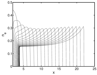
Figure 1: Electron density $n_{e}$ of a planar ionization wave for fixed time intervals vs coordinate $x=z/E_{0}$, in which $z$ is the propagation direction (from the negative to the positive plate) and $E_{0}$ is the modulus of the initial electric field (that is constant) between the plates. The initial data is a compactly supported neutral seed of ionization near the negative plate $x=0$. By using the formulation in terms of the shielding factor we can see that, after evolution, the ionization wave converges to a travelling wave of constant velocity and constant amplitude, called a shock front.

III.2 Analytical computations

The fact that, in the planar case, the integral term in equation (38) does not depend explicitly on $x$ has an interesting consequence: the velocity of the front can be computed directly from the equation for the shielding factor and it is completely determined by the initial condition. Let us assume that the initial density $\rho_{0}(x)$ (for both electron and positive ion densities) decays sufficiently fast as $x$ goes to infinity. Then we can neglect the term $u\rho_{0}(x)$ in (38) for $x\gg 1$ and look for a solution of the resulting equation in the form

$$u(x,t)=f(\xi=x-ct).$$ (42)

Using the equation (38) for the evolution of the shielding factor with this approximations, we obtain the differential equation

$$\frac{df}{d\xi}=\frac{fv(f)}{c-f},$$ (43)

where the quantity $v(f)$ is given by

$$v(f)=\int_{E_{0}f}^{E_{0}}e^{-1/s}ds.$$ (44)

The front of the wave is localized, at a given time, in points in which $f\simeq 1$. In these points, up to first order in $f$, the quantity $v(f)$ results in $v(f)\simeq E_{0}e^{-1/E_{0}}(1-f)$. Inserting these approximations into equation (43), we get

$$\frac{df}{d\xi}=\frac{E_{0}e^{-1/E_{0}}}{c-1}(1-f).$$ (45)

By integrating this expression and using (23) to obtain the electron density, it can be easily seen that physically acceptable solutions of this equation (i.e. positive value of the electron density in all points), correspond only to values of $f$ given by $f\leq 1$ for large $\xi$. From (45), these physical solutions appear only if $c\geq 1$. So that the velocity $c_{z}$ of propagation of the front, in the original $z$ coordinate, satisfies

$$c_{z}\geq E_{0},$$ (46)

in agreement with the result found in Ute .

Moreover, by using this formulation it is also possible to link the asymptotic behavior of the initial condition $n_{e0}$ with the propagation velocity, so that it will be shown that the initial condition determines the velocity of the front. Suppose that the initial condition for the electron density behaves like $n_{e0}\approx Ae^{-\lambda x}$ as $x\rightarrow\infty$. Then, the asymptotic behavior of the travelling wave satisfies

$$n_{e}\simeq Ae^{-\lambda\xi}\;\;\mbox{, as }\xi\rightarrow\infty.$$ (47)

Using the relation (23), this means that the shielding factor $u=f(\xi)$ behaves like

$$f\simeq 1-\frac{A}{\lambda c}e^{-\lambda\xi}\;\;\mbox{, as }\xi\rightarrow\infty.$$ (48)

When this expression is introduced into equation (45), the relation

$$\lambda=\frac{E_{0}\exp(-1/E_{0})}{c-1},$$ (49)

appears. This is the way in which the asymptotic behavior of the initial condition determines the propagation velocity. By using this link, in Fig. 2 we have plotted several travelling wave profiles for different values of $c$. In Fig. 2(left), the shielding factor has been plotted, and in Fig. 2(right), the corresponding electron density, both as a function of $\xi=x-ct$.

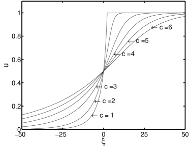
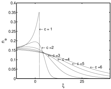
Figure 2: (Left) Electric shielding factor $u$, and (Right) electron density $n_{e}$ of several travelling wave profiles. In the figures, $\xi=x-ct$ and $c$ takes values from $c=1$ (it corresponds to a shock front) to $c=6$. The propagation velocity depends on the way in which the initial electron density behaves as $x$ goes to $\infty$.

As mentioned above, the minimum value of the propagation velocity $c$ of the travelling wave is $c=1$ (it corresponds to $c_{z}=E_{0}$). For this velocity, a shock front can be clearly seen in Fig. 2. Using equation (49), this shock front appears when $\lambda\rightarrow\infty$, so that the initial condition is of compact support, i.e. the initial distribution of charge vanishes strictly beyond a certain point. In Fig. 1, an initial condition fulfilling these requirements has been chosen and a shock front has appeared as predicted by (49). The amplitude of the shock front can be also obtained from equation (45) and is given by

$$n_{e}\simeq E_{0}e^{-1/E_{0}}.$$ (50)

The rest of profiles in Fig. 2 correspond to travelling waves in which the velocity $c$ is larger than 1, so the initial distribution does not have compact support.

III.3 Accelerated fronts

The treatment given above could suggest that ionization fronts always move with constant velocity if the physical setting has planar symmetry. However, it can be shown that fronts with constant velocity appear only if the initial conditions for the particle densities decrease exponentially with the distance from the cathode. In this context, the compactly supported case is treated as an exponential decay with infinite argument, as was done in the previous subsection.

The shielding factor formulation allows us to deduce the existence of accelerated fronts. This situation occurs when taking an initial ionization decaying at infinity slower than an exponential. For instance, by taking

$$n_{e0}\simeq\frac{A}{x^{\alpha}}\;\;\mbox{, \ as }x\rightarrow\infty\ ,$$ (51)

with $\alpha$ positive. Near the front, we can take $u$ close to $1$, so that from equation (38) we get

$$\frac{\partial u}{\partial t}+u\frac{\partial u}{\partial x}=-\frac{A}{x^{\alpha}}u.$$ (52)

If we introduce an expression of the form

$$u=F\left(\xi=\frac{x}{t^{1/\alpha}}\right),$$ (53)

into equation (52), we obtain

$$-\frac{\xi}{\alpha}\frac{\partial F}{\partial\xi}+t^{(\alpha-1)/\alpha}F\frac{\partial F}{\partial\xi}=-\frac{A}{\xi^{\alpha}}F,$$ (54)

which can be approximated by

$$\frac{\xi}{\alpha}\frac{\partial F}{\partial\xi}=\frac{A}{\xi^{\alpha}}F,$$ (55)

when $\alpha<1$ and for large $t$. Hence there might exist fronts whose position is located at the points

$$\frac{x}{t^{1/\alpha}}=C,$$ (56)

implying a superlinear propagation, i.e. an acceleration. This result illustrates the usefulness of our method, showing an unexpected behavior of the well studied planar fronts.

IV Curved symmetries

When the initial particle distributions or the initial electric field do not have planar symmetry, the ionization wave behaves quite differently from what we have described in the previous section. In particular, the amplitude and the velocity of the travelling wave are always not constant. The shielding factor formulation can be applied to those more general curved cases with few changes with respect to the planar case. We will use this formulation to treat the cases of cylindrical and spherical symmetries. In the cylindrical case, we will see that the velocity of the fronts varies in time as $t^{-1/2}$ and the amplitude of the front goes as $1/t$ when the initial conditions for the charged particle densities decay sufficiently fast with the distance to the cathode. In the spherical case, the velocity goes as $t^{-2/3}$ and the amplitude varies as $1/t$ as in the cylindrical case. Both cases can be dealt in a very similar way.

IV.1 Cylindrical symmetry

First we analyze the case with cylindrical symmetry. We consider the experimental situation of two cylindrical plates with radius $r_{0}$ and $r_{1}\gg r_{0}$, respectively. The space between the plates is filled, as in the planar case, with a non-attaching gas. A constant potential difference $V_{0}$ is applied to the plates, so that $V(r_{1})-V(r_{0})=V_{0}>0$. Then the initial electric field ${\bf E}_{0}(r)$ between the plates is

$${\bf E}_{0}(r)=-\frac{B}{r}{\bf u}_{r},\;\;\;B=\frac{V_{0}}{\log{(r_{1}/r_{0})}},$$ (57)

where $B$ is a positive constant and $r$ is the radial coordinate, ranging from $r_{0}$ to $r_{1}$ . An initial neutral seed of ionization $\rho_{0}(r)$ with cylindrical symmetry is taken, so that $n_{e0}(r)=n_{p0}(r)=\rho_{0}(r)$. It is useful to change the spatial variable $r$ to

$$x=\frac{r^{2}}{2B},$$ (58)

so that equation (34) for the shielding factor $u$ takes the form of the Burgers equation

$$\frac{\partial u}{\partial t}+u\frac{\partial u}{\partial x}=-u\rho_{0}(x)-u\int_{\sqrt{B/(2x)}u}^{\sqrt{B/(2x)}}e^{-1/s}ds.$$ (59)

Since the integral term in equation (59) depends explicitly on $x$, it is quite convenient to define the variable $v(x,t)$ through

$$v(x,t)=\int_{\sqrt{B/(2x)}u}^{\sqrt{B/(2x)}}e^{-1/s}ds.$$ (60)

Now, as in the case of planar symmetry, we can integrate (59) along characteristics, transforming this equation into the system of ordinary differential equations

$$\frac{dx}{dt} = u,$$ (61)

$$\frac{du}{dt} = -uv-\rho_{0}(x)u,$$ (62)

Given the definition of $v$ in (60), by taking its time derivative, and using (61) and (62), we close the above system with the equation

$$\frac{dv}{dt} = \frac{\sqrt{B/2}}{2}e^{-\sqrt{2x/B}/u}x^{-3/2}u^{2}$$

$$- \frac{\sqrt{B/2}}{2}e^{-\sqrt{2x/B}}x^{-3/2}u$$

$$+ \sqrt{B/2}e^{-\sqrt{2x/B}/u}x^{-1/2}\left[uv+\rho_{0}(x)u\right].$$

Equations (61), (62), (IV.1), constitute a Lagrangian description of the problem. This dynamical system can be solved with appropriate initial conditions $x(0)=x_{0}$, $u(0)=1$, $v(0)=0$, for any $x_{0}$, allowing us to obtain the profiles for the function $u(x,t)$ at any time $t$.

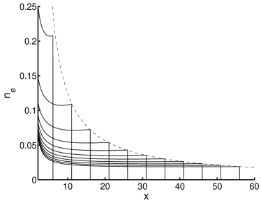
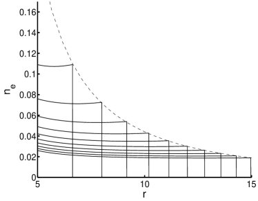
Figure 3: (Left) Electron density $n_{e}$ of an ionization wave with cylindrical symmetry for fixed time intervals vs coordinate $x=r^{2}/(2B)$, where $r$ is the radial coordinate and $B$ is a constant related to the initial electric field between the plates. A compactly supported neutral seed of ionization near the cathode ($x=0$) has been considered as initial condition for the electron density. The solution converges into a shock front with decaying amplitude and constant velocity (in terms of the non-physical $x$ coordinate). The dashed line is the analytical prediction for the amplitude of the shock front. (Right) Same conditions as in (left) but the electron density has been plotted vs the physical radial coordinate $r$. The velocity is clearly non-constant, as explained in the text. The dashed line is the analytical prediction for the amplitude.

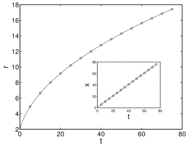
Figure 4: Points are the positions $r$ of the shock front shown in Fig. 3 vs time (in the inset, we plot the positions in terms of $x=r^{2}/(2B)$). Solid lines are, in both cases, the analytical predictions for the position of the shock front as a function of time.

The solutions of the dynamical system given by equations (61), (62), (IV.1), depend on the particular choice of the initial condition for the electron and positive ion densities. In these equations we have used a neutral initial condition given by $n_{e0}(r)=n_{p0}(r)=\rho_{0}(r)$. Consider now the especial case in which the initial condition $\rho_{0}(r)$ for both densities is compactly supported, strictly vanishing beyond a certain point. One example of this behavior is given by a homogeneous thin layer of width $\delta\ll(r_{1}-r_{0})$ from $r=r_{0}$ to $r=r_{0}+\delta$, i.e.

$$\rho_{0}(r)=\left\{\begin{array}[]{ll}\rho_{0}&,\;\;r_{0}<r<r_{0}+\delta\\ 0&,\;\;r_{0}+\delta<r<r_{1}\end{array}\right.$$ (64)

By using this initial condition, we have plotted in Fig. 3 the electron density distribution $n_{e}$ corresponding to a given choice of the physical parameters $V_{0}$, $\rho_{0}$, $\delta$, $r_{0}$ and $r_{1}$. The electron density has been calculated from the shielding factor $u$ using the relation (23) and plotted as a function of $x$ at fixed time intervals. In Fig. 3(left), the electron density has been plotted as a function of coordinate $x$. In Fig. 3(right), it has been plotted as a function of the radial coordinate $r$ with the help of the relation (58). What we can see from the figure is a shock with decaying amplitude, separating the region with charge and the region without charge. The numerical data allows us to measure the velocity of propagation of such front. In Fig. 4, we have plotted the position of the shock $r_{f}$ as a function of time $t$. The velocity of propagation is clearly not constant. However, when we plot the position of the front in terms of $x$, one can observe the following linear relation (see inset Fig. 4),

$$x_{f}(t)=t+x_{0},$$ (65)

which implies, in the original cylindrical variable $r$, an asymptotic behavior such that the position of the front depends on time as

$$r_{f}(t)\simeq\sqrt{2Bt},$$ (66)

so that the velocity of the front behaves as

$$c_{r}(t)\simeq\sqrt{\frac{B}{2t}}.$$ (67)

Using (57) and (66), this result can also be written as

$$c_{r}\simeq E_{0}(r),$$ (68)

showing a close similarity with the case (46) of planar symmetry. Physically, it means that the shock front moves with the drift velocity of electrons as it should be expected.

This behavior can also be obtained analytically, as well as the amplitude of the shock front. This is a considerable advantage of using the formulation in terms of the shielding factor. To do such computation, it is useful to write, locally near the front, the solution for $u$ as

$$u(x,t)=1-a(t)\varphi(\xi),\;\;\xi=x-x_{f}(t).$$ (69)

This expression can be substituted into equation (59). The computation is simplified if we note that the integral term in (59) is very small when $x\gg 1$. We get

$$a(t)\varphi^{\prime}(\xi)-a(t)\varphi^{\prime}(\xi)x^{\prime}_{f}(t)-a^{\prime}(t)\varphi(\xi)+a^{2}(t)\varphi(\xi)\varphi^{\prime}(\xi)\approx 0.$$ (70)

The only way this equation can be satisfied is by choosing

$$x_{f}(t) = t+x_{0}\;,$$ (71)

$$a(t) = \frac{\beta}{(t+t_{0})},$$ (72)

$$\varphi(\xi) = {\beta}^{-1}(x-t-x_{0}),$$ (73)

where $\beta$ is an arbitrary constant depending on initial conditions. Equation (71) is an analytical proof of the numerical law (65) obtained for the position of the front in terms of time. To obtain the amplitude of the shock front, we use relation (23) to compute the electron density from the asymptotic solution (69). What we get is

$$n_{e}(x,t)\simeq\left\{\begin{array}[]{ll}\frac{1}{t+t_{0}}\;\frac{1+(x-t-x_{0})/(t+t_{0})}{1-(x-t-x_{0})/(t+t_{0})}&,\;x\leq t+x_{0}\\ 0&,\;x>t+x_{0}\end{array}\right.,$$ (74)

which implies that the amplitude of the front decays with time as

$$n_{e}(x_{f}(t),t)=\frac{1}{t+t_{0}}.$$ (75)

The analytical curve (75) has been plotted as a dashed line in Figs. 3(left) and 3(right). The agreement with numerical data is seen to be excellent, especially for large times.

IV.2 Spherical symmetry

The physical case in which the initial electric field and the initial particle densities have spherical symmetry shows close similarities with the cylindrical symmetry case. The shielding factor formulation for spherical symmetry has been used in aft to analyze a typical corona discharge. In this example, we have two spherical plates with radius $r_{0}$ and $r_{1}\gg r_{0}$, in which a potential difference $V(r_{1})-V(r_{0})=V_{0}>0$ is applied. Note that, in this case, $r$ is the spherical radial coordinate. The initial seed of ionization is neutral so that $n_{e0}(r)=n_{p0}(r)=\rho_{0}(r)$, and the initial electric field ${\bf E}_{0}(r)$ between the plates is

$${\bf E}_{0}(r)=-\frac{C}{r^{2}}{\bf u}_{r},\;C=V_{0}\frac{r_{0}r_{1}}{r_{1}-r_{0}}.$$ (76)

Changing the spatial variable $r$ to

$$x=\frac{r^{3}}{3C},$$ (77)

the evolution for the screening factor takes the form of the Burgers’ equation

$$\frac{\partial u}{\partial t}+u\frac{\partial u}{\partial x}=-u\rho_{0}(x)-u\int_{u\left(\frac{C}{9x^{2}}\right)^{1/3}}^{\left(\frac{C}{9x^{2}}\right)^{1/3}}e^{-1/s}ds,$$ (78)

where $\rho_{0}(x)$ is the initial distribution of charge. This equation, as in the case of cylindrical symmetry (59), can be integrated along characteristics. The results are very similar to that of cylindrical symmetry shown above aft . For the case of sufficiently localized initial conditions, when the initial electron density strictly vanishes beyond a certain point, there appears a sharp shock with decaying amplitude, separating the region with charge and the region without charge. The velocity of propagation of such front is given by the relation between the position of the front and time: $x_{f}(t)=t+x_{0}$. This implies, in terms of the original variable $r$, an asymptotic behavior

$$r_{f}(t)\simeq(3C)^{1/3}\;t^{1/3},$$ (79)

for the position of the front. The velocity of the front is then

$$c_{r}(t)\simeq\frac{1}{3}(3C)^{1/3}\;t^{-2/3},$$ (80)

or, in terms of the initial electric field (76),

$$c_{r}\simeq E_{0}(r).$$ (81)

The analytical computation of the amplitude and propagation velocity of the shock can be done, by taking the shielding factor near the front as $u(x,t)=1-a(t)\varphi(\xi)$, which gives exactly the same equation found in the cylindrical case (70). The reason of this is that the integral term is neglected in both cases. However, note that the relation between the coordinate $x$ and the physical radial coordinate is different in each case. The position of the front then satisfies $x_{f}(t)=t+x_{0}$ and the amplitude of the electron density front also decays with the law $n_{e}(x_{f}(t),t)=1/(t+t_{0})$. Details and figures showing these results can be found in aft .

V Geometrical diffusion and self-similar behavior

In previous sections we have found that, in the framework of the minimal streamer model without diffusion, when an initial seed of ionization is placed near the cathode, a travelling ionization wave develops towards the anode. The shape and the velocity of this wave depends on the asymptotic behavior of the initial particle (electron and positive ion) density. If the initial particle density is compactly supported, i.e. it vanishes beyond a certain point, then the travelling wave is a shock front, whose velocity is equal to the drift velocity of electrons, i.e. equal to the modulus $E_{0}$ of the initial electric field. This behavior is found in the case in which the physical situation has planar, cylindrical or spherical symmetry. In the last two cases, the velocity, as the initial electric field, is not uniform. With respect to the amplitude of the electron density of the shock, in the planar case, it is constant during the evolution, but it decays as $1/t$ in the curved case (cylindrical or spherical symmetry).

When the initial particle density is not compactly supported, but it does decay exponentially with the distance from the cathode, the shock front does not appear. In the planar case, we have seen that the velocity of the front is then constant and larger than the drift velocity of the electrons, and the amplitude is constant. However, if the initial particle density decay slower than an exponential with the distance from the cathode, accelerated fronts might appear.

Now we are going to investigate the especial features that appear in a case with cylindrical or spherical symmetry when the initial particle densities are not compactly supported but they decay exponentially with the distance from the cathode. We will see that (i) a shock front does not appear, (ii) but a front with an asymptotic self-similar behavior, (iii) whose velocity depends on time in a similar way as the velocity of the shock front seen in the previous section. As a remarkable fact, we will note the appearance of a new type of diffusion effect, due to the geometry of the initial physical situation.

Consider the case of an initial electric field with a cylindrical symmetry as (57). The initial electron and positive ion densities are equal and have cylindrical symmetry, so that $n_{e0}(r)=n_{p0}(r)=\rho_{0}(r)$, where $r$ is the radial coordinate. We use the variable $x=r^{2}/(2B)$ as in the previous section. Now we take an initial neutral charge distribution that is not compactly localized, for example given by

$$n_{e0}(x)=n_{p0}(x)=\rho_{0}(x)\sim e^{-\lambda x},\;\;x\gg 1.$$ (82)

We can solve this problem numerically, integrating along characteristics the dynamical system given by equations (61), (62) and (IV.1). The obtained electron density appears in Fig. 5, shown in constant time intervals, proving that the shock front does not appear. In Fig. 5(left), we plot the electron density vs $x$ for different times. What we see is a travelling wave with increasing thickness and, remarkably, the center of this front moves with constant velocity in the coordinate $x$ in the same way as the shock front does. This means that the velocity of the front center has a similar behavior $c_{r}\sim t^{-1/2}$ that the velocity of the shock front that we analyzed in the previous section. In Fig. 5(right), we plot the electron density vs the radial coordinate $r$.

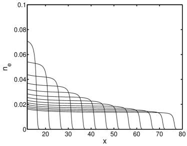
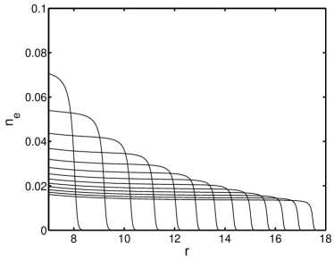
Figure 5: (Left) Electron density $n_{e}$ of an ionization wave with cylindrical symmetry for fixed time intervals vs coordinate $x=r^{2}/(2B)$, where $r$ is the radial coordinate. An initial neutral seed of ionization near the cathode ($x=0$) has been considered such that it exponentially decays with the distance from the cathode. The solution converges into a spreading front with constant velocity in terms of $x$. (Right) Same conditions as in (left) but the electron density has been plotted vs the physical radial coordinate $r$. The velocity is clearly non-constant in terms of $r$.

By using the shielding factor formulation, we can prove that the asymptotic local behavior of the electron density near the front of the travelling wave is self-similar. In order to show this property, we introduce

$$u(x,t)=1-g(x,t),$$ (83)

in the equation (59) describing the evolution of the shielding factor. As we are analyzing the asymptotic behavior, we can take $x\gg 1$ near the front. Keeping the main order terms we obtain the equation

$$\frac{\partial g}{\partial t}+(1-g)\frac{\partial g}{\partial x}=0,$$ (84)

which can be written as

$$\frac{\partial g}{\partial t}-g\frac{\partial g}{\partial\xi}=0,$$ (85)

if we define $\xi=x-t$. Equation (85) is a Burgers equation whose solution $g$ is such that it is constant along the curves given by

$$\frac{d\xi}{dt}=g.$$ (86)

If $g$ varies slowly in some region of size $\delta_{\lambda}$ in space, one can consider $g=G$ at that region, $G$ being a constant. An intermediate asymptotic regime is then obtained, such that it is constant along $\xi=Gt$ and therefore we can assume

$$g(x,t)\simeq g\left(\frac{\xi}{\delta_{\lambda}t}\right).$$ (87)

Hence the asymptotic behavior of the electron density is given by

$$n_{e}=-\frac{1}{u}\frac{\partial u}{\partial t}\simeq\frac{1}{t}\frac{\xi/(\delta_{\lambda}t)}{1+g\left(\xi/(\delta_{\lambda}t)\right)}\frac{d}{d\xi}g\left(\xi/(\delta_{\lambda}t)\right).$$ (88)

Consequently, the asymptotic local behavior of the electron density near the front is self-similar, given by

$$n_{e}(x,t)\simeq\frac{1}{t}f\left(\frac{\xi}{\delta_{\lambda}t}\right),$$ (89)

in which $\xi=x-t$, and $f$ is some universal self-similar profile. Hence the front presents a typical thickness given by

$$\xi_{c}\simeq\delta_{\lambda}t.$$ (90)

This result can be seen in Fig. 6, in which the self-similar character of the asymptotic local behavior is shown. The consequence of this result is clear: even neglecting diffusion, the front spreads out linearly in time when the initial condition for the particle densities decreases exponentially with the distance from the cathode. This is a new and remarkable feature, first considered in aft and explained here, of the curved geometry. It is a diffusive behavior of the solutions of the minimal streamer model caused by the geometry of the electric field. It has been termed geometrical diffusion.

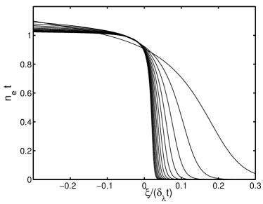
Figure 6: Asymptotic behavior of the electron density shown in Fig. 5. We plot the quantity $n_{e}t$ vs $\xi/(\delta_{\lambda}t)$, and a self-similar behavior is apparent. The front spreads in time, showing a new type of diffusion effect completely due to the geometry of the initial field distribution.

In the spherical case, the same behavior is found, with the only difference being that the $x$ coordinate is related to the radial coordinate $r$ in a different way. We conclude than geometrical diffusion is a universal behavior.

VI Conclusions

The conclusions of this paper are the following. We have made a thorough study of the properties and structure of anode-directed ionization fronts without diffusion, based on a minimal streamer model for non-attaching gases. This model includes impact ionization processes as source terms. The role played by the condition that the magnetic effects in the streamer discharges are neglected has been discussed. As a consequence, it has been proved that an electric shielding factor can be defined, and the physical quantities can be expressed as a function of it.

A Burgers type equation is obtained for the evolution of the electric shielding factor. Thus, the analytical and numerical study of the ionization fronts can be performed by using a Lagrangian formulation. The power of this formulation makes it easier to treat the cases of the non-homogeneous initial electric field in electric discharges with curved symmetries.

We have applied this new formulation to the discharge between planar and curved electrodes (with cylindrical and spherical symmetries). When an initial seed of ionization is placed near the cathode, a travelling wave develops towards the anode. The shape and the velocity of this wave depends on the asymptotic behavior of the initial charged particle densities. If the initial density is compactly supported, then the travelling wave is a shock front, whose velocity is equal to the drift velocity of electrons. This behavior had been predicted for the planar case Ute , but we have found that a similar situation takes place in the case that the physical situation has cylindrical or spherical symmetries. We have derived power laws for the velocity and the amplitude of the shock fronts in the cases of curved symmetry. When we have cylindrical symmetry, the velocity of the shock front behaves as $t^{-1/2}$, and the amplitude behaves as $t^{-1}$. In the spherical case, the velocity of the shock front behaves as $t^{-2/3}$ and the amplitude goes as $t^{-1}$.

When the initial particle density is not compactly supported, but decays exponentially with the distance from the cathode, the shock front does not appear. In the planar case, we have seen that the velocity of the front is then constant and larger than the drift velocity of the electrons, as predicted in Ute . However, if the initial particle density decay slower than an exponential with the distance from the cathode, accelerated fronts appear.

In the cases in which the physical situation has cylindrical or spherical symmetries and the initial ionization seed decays exponentially fast to infinity, we have seen that the velocity follows the same power laws as the compactly supported case. However, the structure of the travelling wave is rather different. We have proved that the asymptotic behavior of the charged particle densities is self-similar. Even if the diffusion has not been considered, the front spreads out linearly in time. This is a remarkable feature, first considered in aft and explained here. It is a diffusive behavior of the solutions of the minimal streamer model caused by the geometry of the electric field, and we have called it geometrical diffusion.

Our analysis opens the way to consider geometrical effects in the stability of ionization fronts.

- (1) Y. P. Raizer, Gas Discharge Physics (Springer, Berlin 1991).
- (2) E. M. van Veldhuizen (ed.), Electrical discharges for environmental purposes: fundamentals and applications (NOVA Science Publishers, New York 1999).
- (3) J. M. Guo and C. H. J. Wu, IEEE Trans. Plasma Sci. 21, 684 (1993).
- (4) S. Chandrasekhar, A. N. Kaufman and K. N. Watson, Ann. Phys. 2, 435 (1957).
- (5) N. Liu and V. P. Pasko, J. Geophys. Res. 109, A04301 (2004).
- (6) U. Ebert, W. van Saarloos and C. Caroli, Phys. Rev. Lett. 77, 4178 (1996); and Phys. Rev. E 55, 1530 (1997).
- (7) S. K. Dhali and P. F. Williams, Phys. Rev. A 31, 1219 (1985); and J. Appl. Phys. 62, 4696 (1987).
- (8) P. A. Vitello, B. M. Penetrante, and J. N. Bardsley, Phys. Rev. E 49, 5574 (1994).
- (9) M. Arrayás, U. Ebert and W. Hundsdorfer, Phys. Rev. Lett. 88, 174502 (2002).
- (10) M. Arrayás and U. Ebert, Phys. Rev. E 69, 036214 (2004).
- (11) A. Rocco, U. Ebert, W. Hundsdorfer, Phys. Rev. E 66, 035102 (2002).
- (12) V. P. Pasko, M. A. Stanley, J. D. Mathews, U. S. Inan and T. G. Wood, Nature 416, 152 (2002).
- (13) U. Ebert, W. van Saarloos, Phys. Rev. Lett. 80, 1650 (1998); Phys. Rep. 337, 139 (2000); and Physica D 146, 1 (2000).
- (14) M. Arrayás, Am. J. Phys. 72, 1283 (2004).
- (15) M. Arrayás, M. A. Fontelos and J. L. Trueba, Phys. Rev. E. 71, 037401 (2005).