On the stability of Bose-Fermi mixtures

Abstract

We consider the stability of a mixture of degenerate Bose and Fermi gases. Even though the bosons effectively repel each other the mixture can still collapse provided the Bose and Fermi gases attract each other strongly enough. For a given number of atoms and the strengths of the interactions between them we find the geometry of a maximally compact trap that supports the stable mixture. We compare a simple analytical estimation for the critical axial frequency of the trap with results based on the numerical solution of hydrodynamic equations for Bose-Fermi mixture.

Experimental realizations of mixtures of degenerate atomic gases have opened exceptional possibilities to investigate fundamental many-body quantum phenomena. The reason is that in such systems there exists a powerful tool (Feshbach resonances) to control the strength of the interaction between atoms. Magnetically tuned scattering resonances allow for changing the magnitude as well as the sign of the scattering length which at low temperatures fully determines the atomic interactions. Recently, mixtures of fermionic gases turned out to be a successful way through in obtaining a molecular Bose-Einstein condensates (BEC) in thermal equilibrium molBEC . Such molecular condensates are good starting points to experimental study of BEC-BCS (Bardeen-Cooper-Schrieffer) crossover region; subject under intensive theoretical investigation. Two-component Fermi gases enabled also getting into a regime of strongly interacting fermionic systems Thomas , here confirmed by the observation of anisotropic expansion of the gas when released from a trap. In Ref. Grimm the pairing gap in a strongly interacting two-component gas of fermionic ⁶Li atoms has been measured showing that the system was already brought in a superfluid state.

Another idea of modifying the interactions between fermions is to immerse Fermi atoms into a Bose gas. In this way a degenerate gas of fermionic potassium (⁴⁰Ka) was forced to collapse by attractive interaction with rubidium (⁸⁷Rb) Bose-Einstein condensate collapse . As it was shown in this experiment, a sufficiently large number of atoms is required to bring a Bose-Fermi mixture to collapse. This result suggests that increasing the attraction between the bosonic and fermionic atoms one can induce the effective attractive interaction between fermions. Increasing the effective fermion-fermion attraction could, on the other hand, lead to a superfluidity in fermionic component. This kind of superfluidity resembles what happens in superconductors where phonon-induced interaction between electrons becomes attractive.

In Ref. BFsol it has been shown (although in a one-dimensional case) that for strong enough attraction between bosons and fermions a Bose-Fermi mixture enters a new phase where both Bose and Fermi components become effectively attractive gases. One of the characteristics of this regime is that it becomes possible to generate bright solitons which are two-component single-peak structures with larger number of bosons than fermions. Since in a three-dimensional space such a mixture might show an instability that could destroy it, it is necessary to investigate in detail the stability-instability crossover. The structure and the instability of the boson-fermion mixtures have been theoretically studied in Ref. Roth , although the analysis was restricted to spherically symmetric systems with equal numbers of atoms in both components. The authors determine, by fitting the numerical data, the expressions for critical numbers of atoms as a function of scattering lengths. In this Letter we investigate the border of the stability region for any trap, find analytic formula for the critical radial trap frequency and compare it with results of numerical solution of hydrodynamic equations describing the Bose-Fermi mixture.

In the mean-field approximation the Bose-Fermi mixture of $N_{B}$ bosons and $N_{F}$ fermions can be described in terms of atomic orbitals FF ; BFsol that fulfill the following set of equations ($j=1,2,...,N_{F}$)

$$i\hbar\,\frac{\partial\varphi^{(B)}}{\partial t}=-\frac{\hbar^{2}}{2m_{B}}\nabla^{2}\varphi^{(B)}+V_{trap}^{(B)}\,\varphi^{(B)}$$

$$+\;g_{B}\,N_{B}\,|\varphi^{(B)}|^{2}\,\varphi^{(B)}+g_{BF}\sum_{i=1}^{N_{F}}|\varphi_{i}^{(F)}|^{2}\,\varphi^{(B)}$$

$$i\hbar\,\frac{\partial\varphi_{j}^{(F)}}{\partial t}=-\frac{\hbar^{2}}{2m_{F}}\nabla^{2}\varphi_{j}^{(F)}+V_{trap}^{(F)}\,\varphi_{j}^{(F)}$$

$$+\;g_{BF}\,N_{B}\,|\varphi^{(B)}|^{2}\,\varphi_{j}^{(F)}$$ (1)

and determine the many-body wave function of the mixture, which is of the form

$$\Psi({\bf x}_{1},...,{\bf x}_{N_{B}};{\bf y}_{1},...,{\bf y}_{N_{F}})=\prod_{i=1}^{N_{B}}\varphi^{(B)}({\bf x}_{i})$$

$$\times\frac{1}{\sqrt{N_{F}!}}\left|\begin{array}[]{lllll}\varphi_{1}^{(F)}({\bf y}_{1})&.&.&.&\varphi_{1}^{(F)}({\bf y}_{N_{F}})\\ \phantom{aa}.&&&&\phantom{aa}.\\ \phantom{aa}.&&&&\phantom{aa}.\\ \phantom{aa}.&&&&\phantom{aa}.\\ \varphi_{N_{F}}^{(F)}({\bf y}_{1})&.&.&.&\varphi_{N_{F}}^{(F)}({\bf y}_{N_{F}})\end{array}\right|$$ (7)

We assume the contact interaction between atoms with $g_{B}$ and $g_{BF}$ being the coupling constants for the boson-boson and boson-fermion interactions, respectively.

Eqs. (1) imply that fermions move under the influence of the effective potential which is the sum of the harmonic trap and the potential that originates in the presence of bosons

$$V_{eff}=V_{trap}^{(F)}+g_{BF}N_{B}|\,\varphi^{(B)}|^{2}\;.$$ (8)

In Fig. 1 we plot this potential (dashed line) as well as the fermionic density (the sum of orbital densities) in the case of one-dimensional system. It is clear from (8) that when the bosons and fermions attract each other strongly enough, the second term in (8) generates the well at the bottom of the harmonic trap (see Fig. 1). Hence, one can distinguish between fermions captured by the bosons (those with energies below zero) and others with higher energies that built broad fermionic basis.

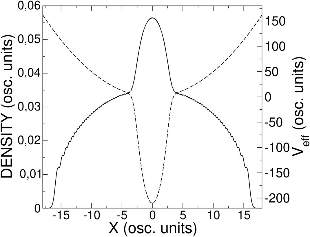
Figure 1: Fermionic density (solid line) normalized to one for a one-dimensional Bose-Fermi mixture of $1000$ bosons and $100$ fermions. The strength of effective repulsion for bosons is $g_{B}=0.0163$ and the attraction between bosons and fermions is determined by $g_{BF}=-0.5$ in oscillatory units. The dashed line shows the effective potential for fermions.

To estimate the number of fermions pulled inside the bosonic cloud we use the Thomas-Fermi approximation. Since we consider the ⁸⁷Rb and ⁴⁰K atoms in a magnetic trap in their doubly spin polarized states, we utilize the relation $m_{F}(\omega_{\alpha}^{F})^{2}=m_{B}(\omega_{\alpha}^{B})^{2}$ (with $\alpha$ equal to $x,y$, and $z$) and rewrite the potential (8) in the following form

$$V_{eff}=\left\{\begin{array}[]{lll}-\frac{|g_{BF}|}{g_{B}}\mu_{B}+(\frac{|g_{BF}|}{g_{B}}+1)\,V_{trap}^{(B)}&&\mbox{inside bosons}\\ &&\\ V_{trap}^{(F)}&&\mbox{\hfill otherwise}\end{array}\right.$$ (12)

where $\mu_{B}$ is the chemical potential for the Bose-Einstein condensate in the Thomas-Fermi limit Stringari

$$\mu_{B}=\frac{\hbar\omega_{ho}}{2}\left(\frac{15\,a_{B}N_{B}}{a_{ho}}\right)^{2/5}\;.$$ (13)

Here, $a_{ho}=\sqrt{\hbar/(m_{B}\omega_{ho})}$ is the harmonic oscillator length and $\omega_{ho}=(\omega_{x}\omega_{y}\omega_{z})^{1/3}$ is the geometric average of the oscillator frequencies. The scattering length $a_{B}$ and the interaction strength $g_{B}$ are related through $g_{B}=4\pi\hbar^{2}a_{B}/m_{B}$.

Now, the number of fermions captured by bosons is just the number of states existing in the potential well defined by the upper branch of (12). Since this potential acts inside the bosonic cloud, one has to count only states with energies below $\frac{|g_{BF}|}{g_{B}}\mu_{B}$ with respect to the minimum of the well. The well itself is the harmonic potential with frequencies multiplied by factors $\sqrt{|g_{BF}|/g_{B}+1}$ in comparison with original ones for bosons. The total number of states in a harmonic potential with the energy less than $\epsilon$ is given by Pethick

$$G(\epsilon)=\frac{\epsilon^{3}}{6\hbar^{3}\,\omega_{x}\omega_{y}\omega_{z}}\;.$$ (14)

Therefore, the number of fermions pulled inside the bosons equals

$$N_{F}^{in}=\frac{\mu^{3}_{B}}{6\hbar^{3}\,\omega_{x}\omega_{y}\omega_{z}}\;\frac{(|g_{BF}|/g_{B})^{3}}{(|g_{BF}|/g_{B}+1)^{3/2}}$$ (15)

and after inserting the chemical potential given by (13) this number becomes

$$N_{F}^{in}=\frac{1}{48}\left(\frac{15\,a_{B}N_{B}}{a_{ho}}\right)^{6/5}\frac{(|g_{BF}|/g_{B})^{3}}{(|g_{BF}|/g_{B}+1)^{3/2}}\;.$$ (16)

Having calculated the number of fermions captured by bosons one can separate off the bosonic component. The energy of the Bose component of a Bose-Fermi mixture in the mean-field approximation reads

$$E = \int\left\{\frac{\hbar^{2}}{2m_{B}}|\nabla\Psi_{B}|^{2}+\frac{m_{B}}{2}[\omega_{\bot}^{2}(x^{2}+y^{2})+\omega_{z}^{2}z^{2}]\,|\Psi_{B}|^{2}\right.$$ (17)

$$+ \left.\frac{1}{2}\,g_{B}|\Psi_{B}|^{4}+g_{BF}|\Psi_{B}|^{2}n_{F}^{in}\right\}\,d^{\,3}r\;,$$

where $\Psi_{B}=N_{B}\varphi^{(B)}$ and $n_{F}^{in}({\bf r})$ is the fermionic density drown into the bosonic cloud. Simplifying the description of the system we introduce the Gaussian variational ansatz for the condensate wave function as well as for the fermionic density

$$\Psi_{B}(\rho,z) = \frac{\sqrt{N_{B}}}{\pi^{3/4}w\sqrt{v}}\exp{\left[-\frac{1}{2}\left(\frac{\rho^{2}}{w^{2}}+\frac{z^{2}}{v^{2}}\right)\right]}$$

$$\sqrt{n_{F}^{in}(\rho,z)} = \frac{\sqrt{N_{F}^{in}}}{\pi^{3/4}w\sqrt{v}}\exp{\left[-\frac{1}{2}\left(\frac{\rho^{2}}{w^{2}}+\frac{z^{2}}{v^{2}}\right)\right]},$$ (18)

where the radial and the axial widths, $w$ and $v$ respectively, are assumed to be the same for both species. This assumption allows for elimination of the fermionic degrees of freedom. Now, the energy of bosons is given by the expression (in oscillatory units based on the axial frequency)

$$\frac{E}{N_{B}} = \frac{1}{2}\left(\frac{1}{2v^{2}}+\frac{1}{w^{2}}\right)+\frac{1}{4}\left(v^{2}+2\beta^{2}w^{2}\right)$$ (19)

$$+ \frac{A}{\sqrt{2\pi\beta}}\frac{1}{vw^{2}}\;,$$

where

$$A=\frac{1}{a_{\bot}}\left(a_{B}N_{B}+a_{BF}N_{F}^{in}\frac{m_{B}}{\mu}\right)\;,$$ (20)

the aspect ratio $\beta=\omega_{\bot}/\omega_{z}$, and the reduced mass $\mu=m_{B}m_{F}/(m_{B}+m_{F})$. The first term in the formula (19) is the kinetic energy of the Bose cloud, the second one describes the harmonic trapping potential whereas the last term covers the interaction between atoms. Since the bosons and fermions attract each other, $a_{BF}$ is negative and when this attraction is strong enough, i.e. in the region of parameters close to the stability border the constant $A$ becomes negative. Therefore, on the edge of the mixture stability the expression (19) can be treated just as the energy of a Bose gas of effectively attractive atoms.

We now find, for a given trap, the maximum strength of attraction between bosons which still allows for the existence of the stable Bose-Einstein condensate. We look for the minimum of the energy (19). The necessary condition for that turns to the set of following equations for the widths

$$-1-\frac{2A}{\sqrt{2\pi\beta}}\frac{1}{v}+\beta^{2}w^{4}=0$$ (21)

$$-\frac{1}{2}+\frac{v^{4}}{2}-\frac{A}{\sqrt{2\pi\beta}}\frac{v}{w^{2}}=0\;.$$ (22)

Calculating $w^{2}$ from the first equation and inserting it in the second one leads to the equation

$$\frac{1}{2}(-1+v^{4})=\frac{A\sqrt{\beta/2\pi}\,v}{\sqrt{1+\frac{2A}{\sqrt{2\pi\beta}}\frac{1}{v}}}\;.$$ (23)

Since $A$ is negative, the Eq. (23) has a solution when the maximum of the right hand side of (23) as a function of the width $v$ is bigger than the value of the left hand side of (23) at the point of this maximum. Then the critical value of the strength $A$ fulfills the biquadratic equation

$$\frac{81}{8\pi^{2}\beta^{2}}A^{4}+\frac{3\sqrt{3}}{2\pi}A^{2}-\frac{1}{2}=0$$ (24)

and the solution

$$|A_{cr}|=\frac{\sqrt{2\pi}}{3^{5/4}}\,\sqrt{-\beta^{2}+\sqrt{3\beta^{2}+\beta^{4}}}\equiv f(\beta)$$ (25)

generalizes well known result for a spherically symmetric trap Stringari .

Equating (20) and (25) one obtains the condition for the parameters of the maximally compact trap which still holds the Bose-Fermi mixture of a given number of atoms and the interaction strengths

$$|a_{BF}|\,\widetilde{N_{F}^{in}}\,\frac{m_{B}}{\mu}\,\beta^{2/5}\,\omega_{z}^{3/5}-a_{B}N_{B}=\sqrt{\frac{\hbar}{m_{B}}}\,\frac{f(\beta)}{\sqrt{\beta\omega_{z}}}\;,$$ (26)

where

$$\widetilde{N_{F}^{in}}=\frac{1}{48}\left(\sqrt{\frac{m_{B}}{\hbar}}15\,a_{B}N_{B}\right)^{6/5}\!\!\frac{(|g_{BF}|/g_{B})^{3}}{(|g_{BF}|/g_{B}+1)^{3/2}}\;.$$ (27)

Solving the condition (26) determines the critical trap frequencies. It turns out that both terms on the left hand side of (26) are much bigger than the term on the right hand side. Therefore, the critical axial trap frequency is given by

$$\omega_{z}^{cr}=\left(\frac{a_{B}N_{B}}{|a_{BF}|\,\widetilde{N_{F}^{in}}}\,\frac{\mu}{m_{B}}\right)^{5/3}\!\!\frac{1}{\beta^{2/3}}\;.$$ (28)

The formula (28) can be also regarded as a way of determining the mutual scattering length $a_{BF}$ when one knows the critical number of bosons (and at the same time the number of drown in fermions is given by (16)) for a particular set of trap parameters. In such a case one has to solve the following equation

$$C\,\omega_{z}^{3/5}\beta^{2/5}\,|a_{BF}|^{4}=(D\,|a_{BF}|+1)^{3/2}\;,$$ (29)

where

$$C=\frac{1}{384N_{B}^{cr}}\frac{1}{a_{B}^{4}}\left(\frac{m_{B}}{\mu}\right)^{4}\left(\sqrt{\frac{m_{B}}{\hbar}}15\,a_{B}N_{B}^{cr}\right)^{6/5}$$

$$D=\frac{1}{2a_{B}}\frac{m_{B}}{\mu}\;.$$ (30)

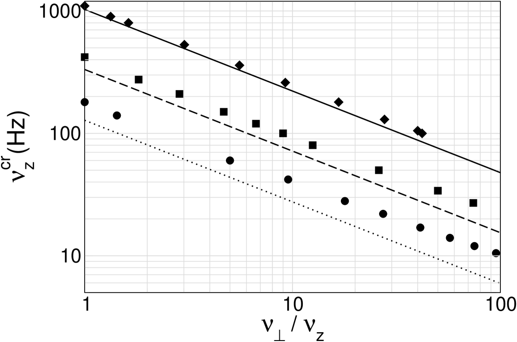
Figure 2: Critical axial frequency as a function of the aspect ratio for the mixture of $10^{4}$ bosons and $10^{4}$ fermions. Points and lines come from the numerical solution of a set of hydrodynamic equations and from the analytical formula (28), respectively. Solid circles (dotted line), squares (dashed line), and diamonds (solid line) correspond to the mutual scattering length $a_{BF}=-21.7$ nm, $-17.6$ nm, and $-13.8$ nm, successively.

In Figs. 2 and 3 we plot $\nu_{z}^{cr}=\omega_{z}^{cr}/(2\pi)$ as a function of the aspect ratio, calculated based on the formula (28). Since there is a controversy over the value of the scattering length $a_{BF}$ collapse ; Simoni ; Jin , we included three different values of it. We show also points obtained from numerical integration of a set of equations that are a hydrodynamic version of Eqs. (1). The hydrodynamic equations can be derived from a set of equations for reduced density matrices (see Ref. Tomek ) after making a local equilibrium assumption for fermions (i.e., utilizing the Thomas-Fermi approximation) and calculating the interaction between bosons and fermions within the mean-field approach. The basic ”objects” in the hydrodynamic approximation are then the condensate wave function and the fermionic density and velocity fields. Hence, the equation for the condensate wave function looks like that in a set of Eqs. (1) but with the last term equal to $g_{BF}n_{F}\varphi^{(B)}$ (with $n_{F}$ being the fermionic density). On the other hand, the equations describing fermions are the usual hydrodynamic equations, i.e., the continuity equation and the Euler-type equation of motion.

Figure 3: The same as in Fig. 2 but for larger number of atoms, here $N_{B}=N_{F}=10^{5}$.

Figs. 2 and 3 show good agreement between the formula (28) and the numerical points for weaker boson-fermion attraction (i.e., less negative scattering length $a_{BF}$). The growing discrepancy for stronger attraction means that the number of fermions pulled inside bosons is overestimated. Indeed, the formula (16) derived based on the Thomas-Fermi approximation for bosons, does not account for the effect of shrinking the bosonic cloud while capturing more and more fermions.

In conclusion, we have analyzed the Bose-Fermi mixture in a regime of parameters, where both gases start to behave as a systems of effectively attractive atoms and the existence of the mixture is in danger due to the possible collapse. We found an analytical formula which determines the parameters of maximally compact trap allowing for the stable mixture. We compare this estimate with the results obtained by solving numerically the hydrodynamic equations describing the Bose-Fermi mixture. It turns out that the collapse is very sensitive to the value of the scattering length $a_{BF}$ and therefore could help to determine this scattering length.

- (1) S. Jochim, M. Bartenstein, A. Altmeyer, G. Hendl, S. Riedl, C. Chin, J.H. Denschlag, R. Grimm, Science 302, 2101 (2003); M. Greiner, C.A. Regal, D.S. Jin, Nature 426, 2101 (2003); M.W. Zwierlein, C.A. Stan, C.H. Schunck, S.M.F. Raupach, S. Gupta, Z. Hadzibabic, and W. Ketterle, Phys. Rev. Lett. 91, 250401 (2003); T. Bourdel, L. Khaykovich, J. Cubizolles, J. Zhang, F. Chevy, M. Teichmann, L. Tarruell, S.J.J.M.F. Kokkelmans, and C. Salomon, Phys. Rev. Lett. 93, 050401 (2004).
- (2) K.M. O’Hara, S.L. Hemmer, M.E. Gehm, S.R. Granade, and J.E. Thomas, Science 298, 2179 (2002).
- (3) C. Chin, M. Bartenstein, A. Altmeyer, S. Riedl, S. Jochim, J. H. Denschlag, R. Grimm, Science 305, 1128 (2004).
- (4) G. Modugno, G. Roati, F. Riboli, F. Ferlaino, R.J. Brecha, and M. Inguscio, Science 297, 2240 (2002).
- (5) T. Karpiuk, M. Brewczyk, S. Ospelkaus-Schwarzer, K. Bongs, M. Gajda, and K. Rza̧żewski, Phys. Rev. Lett. 93, 100401 (2004).
- (6) R. Roth and H. Feldmeier, Phys. Rev. A 65, 021603 (2002); R. Roth, Phys. Rev. A 66, 013614 (2002).
- (7) T. Karpiuk, M. Brewczyk, and K. Rza̧żewski, Phys. Rev. A 69, 043603 (2004).
- (8) C.J. Pethick and H. Smith, Bose-Einstein Condensation in Dilute Gases (Cambridge University Press, New York, 2002).
- (9) F. Dalfovo, S. Giorgini, L.P. Pitaevskii, and S. Stringari, Rev. Mod. Phys. 71, 463 (1999).
- (10) A. Simoni, F. Ferlaino, G. Roati, G. Modugno, and M. Inguscio, Phys. Rev. Lett. 90, 163202 (2003).
- (11) J. Goldwin, S. Inouye, M.L. Olsen, B. Newman, B.D. DePaola, and D.S. Jin, Phys. Rev. A 70, 021601 (2004).
- (12) T. Karpiuk, M. Brewczyk, Ł. Dobrek, M.A. Baranov, M. Lewenstein, and K. Rza̧żewski, Phys. Rev. A 66, 023612 (2002).